
Lecture
An array is a data structure that stores a set of values (array elements) identified by an index or a set of indices taking integer (or integer-convertible) values from some given contiguous range. A one-dimensional array can be viewed as an implementation of the abstract data type vector. In some programming languages, an array may also be called a table, row, vector, or matrix.
The dimensionality of an array is the number of indices needed to unambiguously address an element within the array. By the number of indices used, arrays are divided into one-dimensional, two-dimensional, three-dimensional, and so on.
The shape or structure of an array is the information about the number of dimensions and the size (extent) of the array along each dimension; it can be represented by a one-dimensional array .
A distinctive feature of an array as a data structure (unlike, for example, a linked list) is the constant computational complexity of accessing an array element by index . An array is a random-access data structure.
In the simplest case, an array has constant length in all dimensions and can store data of only one type, specified at declaration. A number of languages also support dynamic arrays , whose length can change while the program is running, and heterogeneous arrays, which can store data of different types in different elements. Some specialized types of arrays used in various languages and implementations are the associative array, segment tree, VList, parallel array, and sparse array.
The main advantages of using arrays are the ease of computing an element's address from its index (since array elements are laid out one after another), equal access time to all elements, and the small size of elements (they consist only of the information field).
Among the drawbacks are the impossibility of deleting or adding an element without shifting the others when using static arrays, and, with dynamic and heterogeneous arrays, lower performance due to the overhead of supporting dynamism and heterogeneity. When working with arrays implemented in the C style (with pointers) and without additional checking facilities, a typical runtime error is the risk of going out of array bounds and corrupting data.
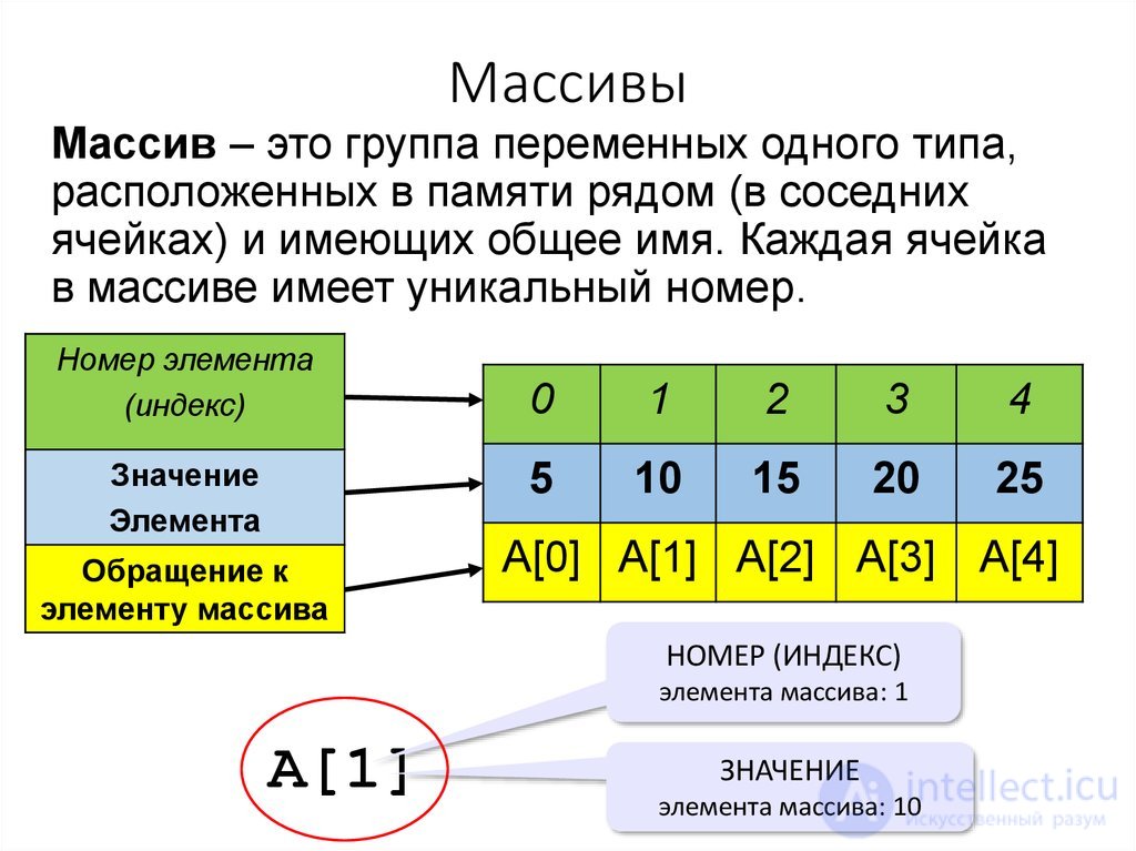
When data objects are stored in an array, individual objects are selected by an index, which is usually a non-negative scalar integer . Indices are also called subscripts. An index maps the array value to a stored object.
There are three ways to index the elements of an array:
0 ( zero-based indexing )
The first element of the array is indexed by index 0.
1 ( one-based indexing )
The first element of the array is indexed by index 1.
n ( n-based indexing )
The base index of an array can be chosen freely. Usually, programming languages that allow n-based indexing also allow negative index values and other scalar data types, such as enumerations or characters , to be used as an array index.
Using zero-based indexing is a design choice of many influential programming languages, including C , Java and Lisp . It leads to a simpler implementation, where the index refers to an offset from the starting position of the array, so the first element has an offset of zero.
Arrays can have multiple dimensions, so it is not uncommon to access an array using multiple indices. For example, a two-dimensional array Awith three rows and four columns can provide access to the element in the 2nd row and 4th column using the expression A in the case of a zero-based indexing system. Thus, two indices are used for a two-dimensional array, three for a three-dimensional array, and n for an n-dimensional array .
The number of indices needed to specify an element is called the dimension, dimensionality, or rank of the array.
In standard arrays, each index is restricted to a certain range of consecutive integers (or consecutive values of some enumerated type ), and the address of an element is computed by a "linear" formula in the indices.
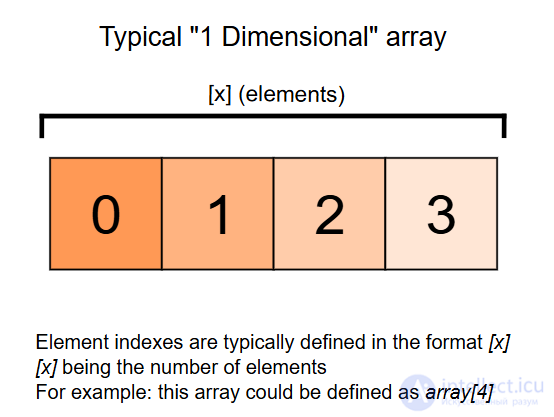
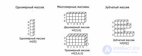
Diagram of a typical one-dimensional array
A one-dimensional array (or array with one dimension) is a type of linear array. Its elements are accessed using a single index, which can represent a row or column index.
As an example, consider the C declaration int anArrayName[10];, which declares a one-dimensional array of ten integers. Here the array can store ten elements of type int. This array has indices ranging from zero to nine. For example, the expressions anArrayName and anArrayName are the first and last elements, respectively.
For a vector with linear addressing, the element with index i is located at the address B + c · i , where B is a fixed base address and c is a fixed constant, sometimes called the address increment or stride .
If the valid element indices begin at 0, the constant B is simply the address of the first element of the array. For this reason, the C programming language specifies that array indices always begin at 0; and many programmers will call that element "zeroth" rather than "first".
However, one can choose the index of the first element by choosing an appropriate base address B. For example, if the array has five elements indexed from 1 to 5, and the base address B is replaced by B + 30 c , then the indices of those same elements will be from 31 to 35. If the numbering does not start at 0, the constant B may not be the address of any element.
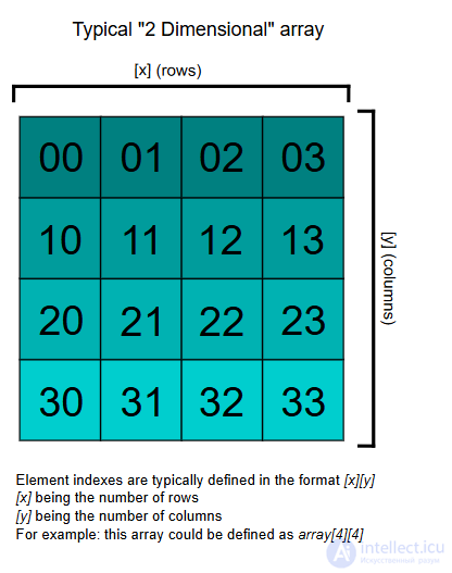
Diagram of a typical two-dimensional array
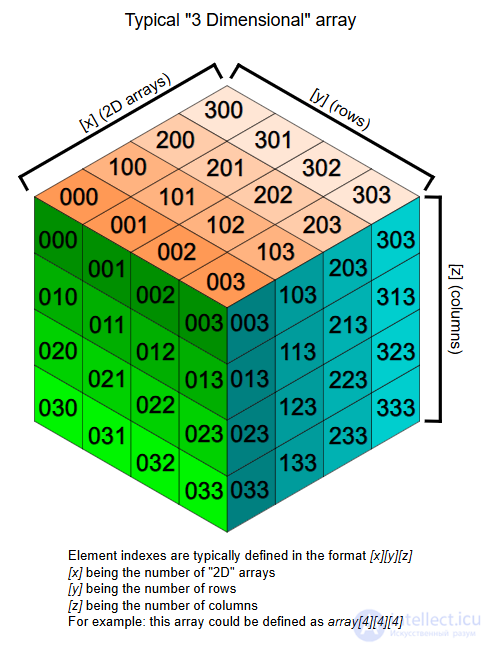
Diagram of a typical 3D array
For a multidimensional array, the element with indices i , j will have the address B + c · i + d · j , where the coefficients c and d are the address increments for the row and column respectively.
More generally, in a k -dimensional array, the address of the element with indices i 1 , i 2 , ..., i k is

For example: int a ;
This means that the array a has 2 rows and 3 columns, and the array is of integer type. Here we can store 6 elements; they will be stored linearly, starting with the first row and then continuing with the second row. The above array will be stored as a 11 , a 12 , a 13 , a 21 , a 22 , a 23 .
This formula requires only k multiplications and k additions for any array that can fit in memory. Moreover, if any coefficient is a fixed power of 2, the multiplication can be replaced by a bit shift .
The coefficients c k must be chosen so that each valid index tuple corresponds to the address of a distinct element.
If the minimum allowed value for each index is 0, then B is the address of the element whose indices are all zero. As in the one-dimensional case, the element indices can be changed by changing the base address B. Thus, if a two-dimensional array has rows and columns indexed from 1 to 10 and from 1 to 20 respectively, then replacing B by B + c 1 − 3 c 2 will renumber them from 0 to 9 and from 4 to 23 respectively. Using this capability, some languages (such as FORTRAN 77) specify that array indices begin at 1, as in mathematical tradition, while other languages (such as Fortran 90, Pascal and Algol) let the user choose the minimum value for each index.
The addressing formula is completely defined by the dimension d , the base address B and the increments c 1 , c 2 , ..., c k . It is often useful to pack these parameters into a record called the array descriptor, stride vector or dope vector . The size of each element, as well as the minimum and maximum values allowed for each index, may also be included in the dope vector. The dope vector is a complete descriptor of the array and a convenient way of passing arrays as arguments to procedures . Many useful array slicing operations (such as selecting a subarray, swapping indices or reversing the direction of the indices) can be performed very efficiently by manipulating the dope vector.
Often the coefficients are chosen so that the elements occupy a contiguous area of memory. However, this is not necessary. Even if arrays are always created with contiguous elements, some array slicing operations may create non-contiguous subarrays from them.
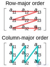
Illustration of row-major and column-major order
There are two systematic compact layouts for a two-dimensional array. For example, consider the matrix
A=[123456789].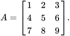
In row-major layout (adopted in C for statically declared arrays), the elements in each row are stored in consecutive positions, and all the elements of a row have a lower address than any of the elements of the next row:
| 1 | 2 | 3 | 4 | 5 | 6 | 7 | 8 | 9 |
In column-major order (traditionally used in Fortran), the elements in each column are laid out consecutively in memory, and all the elements of a column have a lower address than any of the elements of the next column:
| 1 | 4 | 7 | 2 | 5 | 8 | 3 | 6 | 9 |
For arrays with three or more indices, "row-major order" puts in consecutive positions any two elements whose index tuples differ only by one in the last index. "Column-major order" is analogous with respect to the first index.
In systems that use a processor cache or virtual memory , scanning an array is much faster if consecutive elements are stored in consecutive memory positions rather than scattered. This is known as spatial locality, which is a type of locality of reference . Many algorithms that use multidimensional arrays will scan them in a predictable order. A programmer (or a sophisticated compiler) can use this information to choose between row-major and column-major layout for each array. For example, when computing the product A · B of two matrices, it would be best to store A in row-major order and B in column-major order.
Static arrays have a fixed size when they are created and therefore do not allow inserting or deleting elements. However, by allocating a new array and copying the contents of the old array into it, a dynamic version of an array can be implemented efficiently; see dynamic array . If this operation is performed infrequently, insertions at the end of the array require only amortized constant time.
Some array data structures do not reallocate memory but keep a count of the number of array elements in use, called the count or size. This effectively makes the array a dynamic array with a fixed maximum size or capacity; Pascal strings are examples of this.
Sometimes more complex (non-linear) formulas are used. For example, for a compact two-dimensional triangular array, the addressing formula is a polynomial of degree 2.
An array is an ordered collection of elements, each of which stores one value identified by one or more indices. In the simplest case, an array has a constant length and stores data items of the same type, and the indices are integers.
The number of indices used by an array can vary: arrays with one index are called one-dimensional, with two — two-dimensional, and so on. A one-dimensional array corresponds loosely to a vector in mathematics; a two-dimensional one ("row", "column") corresponds to a matrix. Arrays with one or two indices are used most often; those with three less often; even more indices are encountered extremely rarely.
Depending on the programming language, the first element of an array may have a different index. Three main varieties of arrays are distinguished: zero-based, one-based, and based on a specific value set by the programmer (n-based). Zero-based counting is more characteristic of low-level programming languages, although it is also found in high-level languages; for example, it is used in almost all languages of the C family. In a number of languages (Pascal, Ada, Modula-2) the index range can be defined as an arbitrary range of values of any data type that can be converted to an integer, that is, integers, characters, enumerations, even the Boolean type (in the latter case the array has two elements, indexed by the values "True" and "False").
Example of a fixed array in Pascal
    {One-dimensional array of integers.  Elements are numbered from 1 to 15}
  a: array [1..15] of Integer;
    {Two-dimensional array of characters.  Columns are numbered by type Byte (from 0 to 255)
     rows from 1 to 5}
  multiArray : array [Byte, 1..5] of Char;
    {One-dimensional array of strings.     Numbering by type word (from 0 to 65536)}
  rangeArray : array [Word] of String;
Example of a fixed array in C
  int Array[10];         // One-dimensional array: of integers, size 10;
                         // Elements are numbered from 0 to 9.

  double Array[12][15];  // Two-dimensional array:
                         // of double-precision real numbers,
                         // of size 12 by 15;
                         // Numbering: rows — from 0 to 11,
                         // columns — from 0 to 14.
In some programming languages, multidimensional arrays are built from one-dimensional ones whose elements are arrays .
Example of a two-dimensional array in JavaScript
    //Creating a two-dimensional array of numbers:
    var array = [
        [11, 12, 13, 14, 15, 16], // First row-array
        [21, 22, 23, 24, 25, 26], // Second
        [31, 32, 33, 34, 35, 36]  // Third
    ];

    // Printing the array to the console:
    array.forEach((subArray) => {   // For each sub-array,
       subArray.forEach((item) => { // for each of its elements,
           console.log(item);       // — print that element to the console.
       });
    });
Support for indexed arrays (their own declaration syntax, functions for working with elements, and so on) is present in most high-level programming languages. The maximum permitted dimensionality of an array, the types and ranges of index values, and the restrictions on element types are determined by the programming language or the particular translator.
In programming languages that allow programmers to declare their own types, it is usually possible to create an "array" type. The definition of such a type specifies the types and/or ranges of values of each of the indices and the type of the array elements. The declared type can subsequently be used to define variables, formal parameters and function return values. Some languages support assignment operations for array variables (where a single operation assigns to all elements of the array the values of the corresponding elements of another array).
Declaring an "array" type in Pascal
  type
    TArrayType = array [0..9] of Integer;
    (* Arrays with the given parameters:
        1. Size — 10 cells;
        2. Type of elements that can be stored —
                — integers in the range [−32,768; 32,767],
        — are declared with an operand type called "TArrayType". *)
  var
    arr1, arr2, arr3: TArrayType;
    (* Declaration of three array variables of the same type
        (the "TArrayType" above). *)
In the APL programming language, the array is the fundamental data type (a zero-dimensional array is called a scalar, a one-dimensional array a vector, and a two-dimensional array a matrix) . In addition to array assignment, this language supports vector and matrix arithmetic operations, each performed by a single command, operations for shifting data in arrays, and sorting of matrix rows.
Dynamic arrays are arrays whose size can change while the program is running. Ordinary (non-dynamic) arrays are also called fixed or static arrays.
Dynamic arrays can be implemented either at the level of the programming language or at the level of system libraries. In the latter case, the dynamic array is an object of the standard library, and all operations on it are implemented within that same library. Either way, support for dynamic arrays presupposes the following capabilities:
Example of constructs for working with dynamic arrays in Delphi:
var  // Declarations of dynamic arrays
  byteArray  : Array of Byte;           // One-dimensional array
  multiArray : Array of Array of string;  // Multidimensional array
...
  SetLength(byteArray, 1); // Set the array size to 1 element.
  byteArray[0] := 16;       // Write an element.
  SetLength(byteArray, Length(byteArray)+1); // Increase the array size by one
  byteArray[Length(byteArray) - 1] := 10;    // Write a value to the last element.
  WriteLn(byteArray[Length(byteArray) - 1]); // Print the last element of the array.
...
  SetLength(multiArray, 20, 30); // Set the size of the two-dimensional array
  multiArray[10,15] := 12;       // Write a value
  SetLength(multiArray, 10, 15); // Reduce the size
  WriteLn(Length(multiArray), '  ', Length(multiArray[0])
A heterogeneous array is one in whose different elements values belonging to different data types can be written directly. An array that stores pointers to values of various types is not heterogeneous, since the data actually stored in the array belong to a single type — the "pointer" type. Heterogeneous arrays are convenient as a universal structure for storing collections of data of arbitrary types. Implementing heterogeneity requires a more complex array support mechanism in the language translator. In a number of programming languages, heterogeneous arrays are called records.
The typical way to implement a static homogeneous array (one that stores data of a single type) is to allocate a contiguous block of memory of size  , where S is the size of one element, and
  are the sizes of the index ranges (that is, the number of values that the corresponding index can take). When accessing an array element with index
 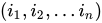 , the address of the corresponding element is computed as
  , where B is the base (the address of the start of the array's memory block), and
  is the value of the k-th index, converted to an integer with a zero starting offset. The order of the indices in the address calculation formula may vary. (This method corresponds to the implementation in most C compilers; in Fortran the order of the indices is the opposite ).
Thus, the address of an element with a given set of indices is computed in such a way that, from a theoretical point of view, the access time to all elements of the array is the same; however, different response latencies of main memory for cells located in different memory units may have an effect, but in high-level programming practice such subtleties are, with rare exceptions, ignored.
The usual way to implement heterogeneous arrays is to store the element values separately and to place pointers to these elements in the array's memory block (organized as an ordinary homogeneous array, described above). Since pointers to values of any types usually have the same size, the simplicity of address calculation is preserved, although additional overhead arises for allocating the element values and accessing them.
For dynamic arrays, the same allocation mechanism as for static ones can be used, but with some amount of extra memory allocated for expansion, and with added mechanisms for resizing and moving the array's contents in memory.
Dynamic and heterogeneous arrays can also be implemented using fundamentally different methods of storing values in memory, for example singly or doubly linked lists. Such implementations can be more flexible but, as a rule, require additional overhead. Moreover, they usually cannot meet the requirement of constant-time access to an element.
The dimension of an array is the number of indices needed to select an element. Thus, if the array is viewed as a function on the set of possible index combinations, this is the dimension of the space of which its domain is a discrete subset. Thus, a one-dimensional array is a list of data, a two-dimensional array is a rectangle of data, [ 12 ] a three-dimensional array is a block of data, and so on.
This should not be confused with the dimension of the set of all matrices with a given domain, that is, with the number of elements in the array. For example, an array with 5 rows and 4 columns is two-dimensional, but such matrices form a 20-dimensional space. Similarly, a three-dimensional vector can be represented by a one-dimensional array of size three.
| Peek (index) |
Mutate (insert or delete) at … | Excess space, average |
|||
|---|---|---|---|---|---|
| Beginning | End | Middle | |||
| Linked list | Θ( n ) | Θ(1) | Θ(1) — known end element; Θ( n ), unknown end element |
Θ( n ) | Θ( n ) |
| Array | Θ(1) | — | — | — | 0 |
| Dynamic array | Θ(1) | Θ( n ) | Θ(1) amortized | Θ( n ) | Θ( n ) [ 9 ] |
| Balanced tree | Θ(log n) | Θ(log n) | Θ(log n ) | Θ(log n ) | Θ( n ) |
| Random-access list | Θ(log n) [ 10 ] | Θ(1) | — [ 10 ] | — [ 10 ] | Θ( n ) |
| Hashed array tree | Θ(1) | Θ( n ) | Θ(1) amortized | Θ( n ) | Θ(√ n ) |
Dynamic arrays or growable arrays are similar to arrays but add the ability to insert and delete elements; adding and deleting at the end is particularly efficient. However, they reserve linear ( Θ ( n )) additional storage, whereas arrays do not reserve additional storage.
Associative arrays provide a mechanism for array-like functionality without the huge storage overhead when the index values are sparse. For example, an array containing values only at indices 1 and 2 billion may benefit from using such a structure. Specialized associative arrays with integer keys include Patricia tries , Judy arrays and van Emde Boas trees .
Balanced trees require O(log n ) time for indexed access, but also allow inserting or deleting elements in O(log n ) time , whereas growable arrays require linear (Θ( n )) time to insert or delete elements at an arbitrary position.
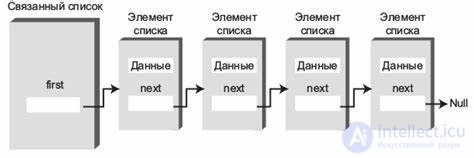
Linked lists allow constant-time removal and insertion in the middle, but require linear time for indexed access. Their memory use is typically worse than that of arrays, but still linear.
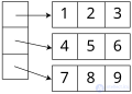
An Iliffe vector is an alternative to a multidimensional array structure. It uses a one-dimensional array of references to arrays of one dimension less. For two dimensions, in particular, this alternative structure would be a vector of pointers to vectors, one for each row (a pointer to c or c++). Thus an element in row i and column j of an array A would be accessed by double indexing ( A [ i ][ j ] in typical notation). This alternative structure allows jagged arrays , where each row may have a different size — or, in general, where the valid range of each index depends on the values of all preceding indices. It also saves one multiplication (by the column address increment), replacing it with a bit shift (to index the vector of row pointers) and one extra memory access (fetching the row address), which may be worthwhile on some architectures.
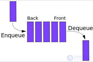
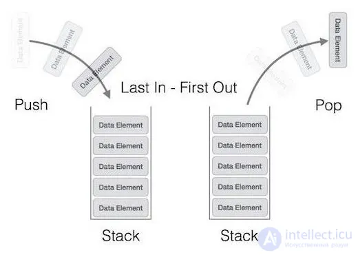
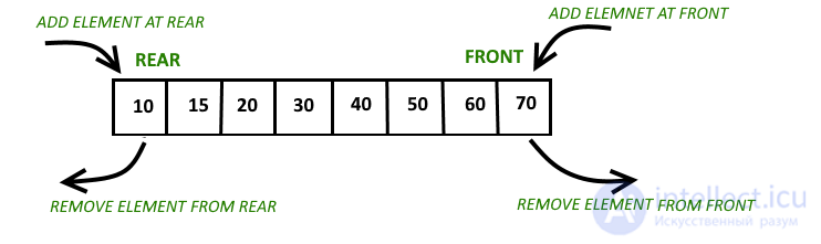
| Characteristic | Queue | Stack | Linked List | Array | Deque | Heap |
|---|---|---|---|---|---|---|
|
Principle of operation
|
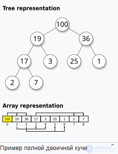
FIFO (first in — first out) | LIFO (last in — first out) | Elements are linked by pointers | Indices are fixed | Access to both ends | A tree where the parent is >= (max heap) or <= (min heap) its children |
|
Adding elements
|
At the end (enqueue) | At the end (push) | At the beginning or end | At any position | At the beginning or end | At the root (with rebalancing) |
|
Removing elements
|
From the beginning (dequeue) | From the end (pop) | At any position (requires traversal) | At any position (but requires shifting) | At the beginning and end | From the root (with reordering) |
|
Accessing elements
|
Only the first (head) | Only the last (top) | Sequential (via links) | Direct access by index | At the beginning and end | Only the root (the largest or smallest element) |
|
Running time (average)
|
O(1) (add/remove) | O(1) (add/remove) | O(1) (add at the beginning/end) | O(1) (access), O(n) (insert/remove) | O(1) (operations at the ends) | O(log n) (add, remove, access to the root) |
| Where it is used | Background tasks, thread management, BFS algorithms | Recursion, undoing actions (Ctrl+Z) | Dynamic structures, graph traversal | Static structures, fast access | Buffers, parsers, data processing | Priority queues, Dijkstra's and Huffman's algorithms, storing classes |
 |
 |
 |
 |
 |
 |


Comments