Lecture
The chain of Markov is a sequence of random events with a finite or countable number of outcomes, characterized by the property that, speaking loosely, with a fixed present, the future is independent of the past. Named in honor of A. A. Markov (senior).
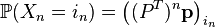
Sequence of discrete random variables  called a simple Markov chain (with discrete time) if
 .
.
Thus, in the simplest case, the conditional distribution of the subsequent state of the Markov chain depends only on the current state and does not depend on all previous states (unlike the Markov chains of higher orders).
Range of values of random variables  called the chain space , and the number
  - step number.
Matrix  where
where

is called the matrix of transition probabilities on  m step and vector
  where
where
- the initial distribution of the Markov chain.
Obviously, the transition probability matrix is stochastic, that is,
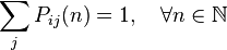 .
.
A Markov chain is said to be single -pitch if the transition probability matrix does not depend on the step number, that is,
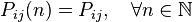 .
.
Otherwise, the Markov chain is called inhomogeneous. In the following, we will assume that we are dealing with homogeneous Markov chains.
From the properties of conditional probability and the definition of a homogeneous Markov chain we get:
 ,
,
whence the special case of the Kolmogorov – Chapman equation follows:
 ,
,
that is, the transition probability matrix for steps of a homogeneous Markov chain -th degree of the matrix of transition probabilities for 1 step. Finally,
 .
.
Family of discrete random variables  called a Markov chain (with continuous time) if
 .
.
A chain of Markov with continuous time is called homogeneous if
 .
.
Similar to the discrete time case, the finite-dimensional distributions of a homogeneous Markov chain with continuous time are completely determined by the initial distribution

and the matrix of transition functions ( transition probabilities )
 .
.
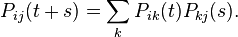
The matrix of transition probabilities satisfies the Kolmogorov – Chapman equation: 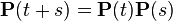 or
or
By definition, the intensity matrix 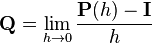 or equivalently
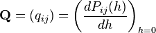 .
.
From the Kolmogorov-Chapman equation, two equations follow:
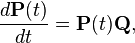
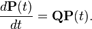
For both equations, the initial condition is chosen  . Appropriate solution
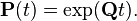
For anyone  matrix
  has the following properties:
non-negative:  (nonnegative probability). equals 1:
  (total probability), that is, the matrix is stochastic on the right (or in rows).
 matrices do not exceed 1 in absolute value:
  . If a
  then
then  . matrices corresponds to at least one non-negative left eigenvector line (equilibrium):


 . matrices all root vectors are proper, that is, the corresponding Jordan cells are trivial.
Matrix  has the following properties:
non-negative:  . non-positive:
  . equals 0:
 matrices non-positive:
  . If a
  then
then 
 matrices corresponds to at least one non-negative left eigenvector line (equilibrium):
  matrices all root vectors are proper, that is, the corresponding Jordan cells are trivial.
For a Markov chain with continuous time, an oriented transition graph (briefly, a transition graph) is constructed according to the following rules:
 connected by oriented edge
  , if a
  (i.e. the flow rate from
  th state in
  is positive.
Topological properties of the transition graph associated with the spectral properties of the matrix . In particular, the following theorems are true for finite Markov chains:
A. For any two different vertices of the transition graph there is such a vertex  a graph (“common drain”) that there are oriented paths from the top to the top and from the top to the top . Note : possible case
  or
or  ; in this case, the trivial (empty) path from to or from to also considered an oriented way.
B. Zero eigenvalue of the matrix nondegenerate.
B. When  matrix tends to the matrix, in which all the rows coincide (and coincide, obviously, with the equilibrium distribution).
A. The transition graph of a chain is oriented.
B. Zero eigenvalue of the matrix is non-degenerate and corresponds to a strictly positive left eigenvector (equilibrium distribution).
B. For some matrix strictly positive (i.e.  for all
  ).
).
G. For all matrix strictly positive.
D. When matrix tends to a strictly positive matrix, in which all the rows coincide (and obviously coincide with the equilibrium distribution).
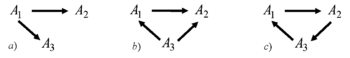
 ); b) weakly ergodic, but not ergodic chain (transition graph is not oriented connected); c) ergodic chain (transition graph orientedly connected).
Let us consider Markov chains with three states and with continuous time, corresponding to the transition graphs shown in Fig. In case (a), only the following nondiagonal elements of the intensity matrix are nonzero:  in case (b) are non-zero only
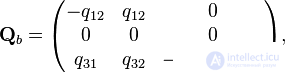
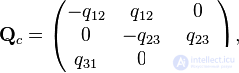
  , and in case (c) -
  . The remaining elements are determined by the properties of the matrix. (the sum of the elements in each row is 0). As a result, for graphs (a), (b), (c), the intensity matrices are:
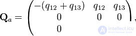
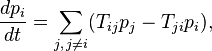
The basic kinetic equation describes the evolution of the probability distribution in a Markov chain with continuous time. The “basic equation” here is not an epithet, but a translation of the term English. Master equation . For a probability distribution vector string  the basic kinetic equation is:

and coincides, essentially, with the direct Kolmogorov equation. In the physical literature, probability column vectors are used more often and the basic kinetic equation is written in the form that explicitly uses the law of conservation of total probability:
Where 
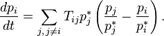
If for the basic kinetic equation there is a positive equilibrium  then it can be written in the form
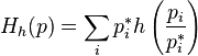
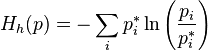
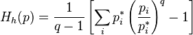
For the basic kinetic equation, there exists a rich family of convex Lyapunov functions — monotonously varying with time distribution probability functions. Let be 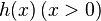 - convex function of one variable. For any positive probability distribution (
  ) we define the function Morimoto
  :
:
 .
.
Derivative on time if  satisfies the basic kinetic equation, there is
 .
.
The last inequality holds because of the bulge  .
.
[edit] ,
,  ;
;this function is the distance from the current probability distribution to the equilibrium in  -norm The time shift is a contraction of the space of probability distributions in this norm. (For compression properties, see the Banach Fixed Point Theorem article.)
 ,
,  ;
;this function is (minus) Kullback entropy (see Kullback – Leibler Distance). In physics, it corresponds to the free energy divided by  (Where —Permanent Boltzmann,
  - absolute temperature):
if a  (Boltzmann distribution), then
 .
.
 ,
,  ;
;
 ,
,  ;
;this is a quadratic approximation for the (minus) Kullback entropy near the equilibrium point. Up to a time-constant term, this function coincides with the (minus) Fisher entropy, which is given by the following choice,
 ,
,  ;
;this is (minus) Fisher entropy.
 ,
,  ;
;This is one of the analogues of free energy for the entropy of Tsallis. Tsallis entropy
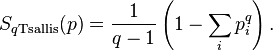
serves as the basis for the statistical physics of nonextensive quantities. With  it tends to the classical Boltzmann – Gibbs – Shannon entropy, and the corresponding Morimoto function to the (minus) Kullback entropy.

Comments
To leave a comment
probabilistic processes
Terms: probabilistic processes