
Lecture 19 min.
Knot theory, to which this special course is devoted, arose
as a mathematical theory at the end of the 18th and the beginning of the 19th century; over
more than a hundred years it was studied by such outstanding mathematicians
as A. T. Vandermonde, C. F. Gauss (who found a remarkable
electromagnetic formula for computing the linking number [37]),
F. Klein, and later M. Dehn [28]. Its systematic exposition
began in the 1880s, when mathematicians and physicists began
compiling tables of knots under the influence of the ideas of the physicist W. Thomson
(later known as Lord Kelvin), who believed that
knots should correspond to chemical elements. However, the real
breakthroughs in knot theory began in the second half of the 20th century and are associated
first of all with the names of J. H. Conway, V. Jones and V. A. Vassiliev,
and later M. L. Kontsevich, V. G. Turaev and M. N. Goussarov.
Knot theory stems from a beautiful and, at first glance, very
simple topological problem, the solution of which, as it turned out,
requires a very complex and deep mathematical apparatus
connected with topology, the theory of discriminants, group theory and Lie algebras,
the theory of multiplicative integrals, tensor algebra, and others.
Moreover, the subject of knots is developing rapidly; in
recent years important works in knot theory (Jones, Witten, Drinfeld
in 1990, Kontsevich in 1998) were recognized with Fields Medals.
In addition, knot theory serves for constructing other theories,
a bright example of which is the Kirby calculus, a theory of
encoding three-dimensional manifolds.
So, let us begin with the definition of a knot. By a knot we will mean a
continuous embedding of the circle S1 into the space R3 (or into the
sphere S3). Visually, a knot can be imagined as a rope with its ends joined together.
We may deform the space R3
(respectively S3), and the knot will move and stretch (but not tear!)
and remain non-self-intersecting. More rigorously, two knots are called
isotopic if one of them can be transformed into the other by a smooth
homeomorphism of the ambient space R3 or S3 onto itself, homotopic to the
identity map in the class of smooth homeomorphisms. Here
we would like to know which knots are isotopic and which are not isotopic.
This problem is called the knot recognition problem. One can speak
of isotopy classes of knots. One can also speak of knot invariants,
that is, functions on isotopy classes of knots, or functions
on knots that do not change under isotopies of knots.
A special case of the knot recognition problem is the problem of
recognizing the trivial knot, which is the simplest knot
(a knot that bounds a disk embedded in three-dimensional
space).
Both of these questions, seemingly very simple at first glance, are very
difficult. In fact, by now these problems have already been solved,
but their solution fills a huge book [41], is
algorithmically complex and is very hard to read. The main stages of the solution of
this problem can be found in the article [116].
In this course we will try to partially answer the question
of the isotopy and non-isotopy of knots. As a rule, in order to
establish the isotopy of knots, one needs to transform one knot into the other by
means of some transformations (for example, Reidemeister moves,
which will be discussed later), while to establish non-isotopy
it suffices to find an invariant that distinguishes these knots.
Knots are usually depicted in the following way. Let a knot be given,
that is, a map f : S1 —► R3 be specified. Consider some plane
h ⊂ R3 and the projection of the knot (strictly speaking, the projection of the image of the function f)
onto this plane. For a plane in general position, that is, "almost
always", this projection will be a graph embedded in the plane
with vertices of valency four. At each vertex
of the graph (which can also be called a crossing) the images of the
projections of different arcs ("pieces") of the knot intersect, and if we specify a
direction x perpendicular to h, then for each such vertex we can
say which arc passes above and which passes below (whose x coordinate is
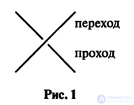
greater and whose is smaller). We mark this on the plane as shown
in Fig. 1.
These types of symbolic depiction of knot arcs
are called, respectively, overcrossings and undercrossings, and such a graph with
overcrossings and undercrossings is called a planar diagram of the knot. Correspondingly, a
four-valent graph without indication of overcrossings and undercrossings
is called the shadow of the knot.
The minimal number of crossings of a planar diagram for
a given isotopy class of a knot is called the complexity of the knot.
So, every knot admits some planar diagram with
overcrossings and undercrossings. A natural question then arises:
have we not lost some information about the knot by encoding
it in this way?
One can easily do the following
Exercise 0.1. Knots having as planar diagrams
isomorphic graphs with identically placed overcrossings and undercrossings
are isotopic.
Let us give several examples.
Example 0.1.
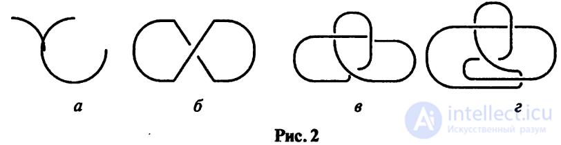
A knot isotopic to a knot having a diagram without crossings (Fig. 2a)
is called the trivial knot. Fig. 2b shows another planar
diagram of the trivial knot. The knot in Fig. 2c is called the trefoil, and the knot
in Fig. 2d is called the figure-eight. Both of these knots are nontrivial, and they
are not isotopic to each other.
For each knot one can construct its mirror image,
the knot obtained by reflecting the given one with respect to some
plane. The diagrams of the mirror image are obtained by replacing
in the diagrams of the original all types of crossings (overcrossings by
undercrossings and vice versa). A knot is called amphichiral if it is isotopic to its
mirror image.
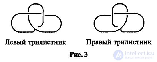
Example 0.2. The trefoil is not an amphichiral knot (the proof
will be given later).
Thus, one can speak of two trefoils, the right-handed
and the left-handed.
Exercise 0.2. Show that the figure-eight is an amphichiral knot.
In many problems of knot theory, oriented
knots are considered: knots on which a direction of traversal is specified, or else
maps of an oriented circle into R3. In this case, an isotopy of knots
is required to preserve orientation.
Alongside knot theory, link theory also developed,
having much in common with knot theory in its approaches. By a
link we will mean a sufficiently smooth embedding of several
circles into R3, requiring that the images of different points of
one and of different circles do not coincide. Each knot,
being the image in R3 of one of the circles, is called a
component of the link. The isotopy of links is naturally defined
(by means of a smooth homeomorphism of the ambient
space), as are planar diagrams of links and link invariants. In
this case, to specify an oriented link one needs to orient all
of its components. There is also another approach to the isotopy of links, in
which during the "isotopy" each component of the link
is allowed to intersect itself, but different components may not intersect.
One can read about this in the remarkable paper [68] by John Milnor,
who introduced the so-called μ-invariants for classifying
links up to such an "isotopy". A trivial link of n
components is a link isotopic to a link whose diagram
consists of n circles (without crossings).
Example 0.3.
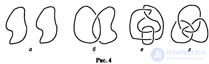
Fig. 4a shows a trivial link of two components.
Figure 46 (b, c, d) shows links called the Hopf link,
the Whitehead link, and the Borromean rings, respectively. The first two links
are named after the topologists H. Hopf and J. Whitehead, and the third after
the Italian Borromeo family, on whose coat of arms it was depicted. All
of them are nontrivial (this will be shown below, once we learn how to compute
the values of invariants that distinguish knots or links), and it is easy to
notice that any two of the three circles are mutually "unlinked".
Let us say a little about invariants. The very first and
simplest invariant of knots and links was the fundamental
group of the knot (link) complement, to which a separate
lecture will be devoted. This invariant is purely topological, and
it is very strong, i.e., it distinguishes knots well (in particular,
the trivial knot and the trivial link with any number of components),
but it does not distinguish some non-isotopic links. Moreover, such a
"solution" to the knot recognition problem is not complete, since
it reduces to the, generally speaking, unsolvable problem of recognizing
groups given by generators and relations.
In 1923 the American mathematician Alexander in his papers
[2, 3] introduced a polynomial invariant of knots and links, based
on the fundamental group of the knot complement.
Then in 1932 the book "Knotentheorie" by the German topologist
Reidemeister was published, in which the Alexander invariant was described,
a list of Reidemeister moves was given, and the theorem was proved
that any two planar diagrams give isotopic
knots only if there exists a chain of moves from one
diagram to the other; the book also gave a table of isotopy classes of
knots of complexity up to seven inclusive. There is also an English
translation of this book [79]. To prove the invariance of a given
function on knots, one usually checks its invariance
under the Reidemeister moves.
Among the books containing information on knots "of those times", I note
the books by Crowell and Fox (in Russian) [104], as well as Burde
and Zieschang [19].
Surveys of low-dimensional topology and knot theory can be found
in [130, 129].
The next stage in the theory of knots and links was the
discovery of the Conway polynomial, see [25], based on the so-called skein
relations, or Conway-type relations, which is
combinatorial and based on the notion of a planar knot diagram. The
Alexander polynomial could also be interpreted in terms of Conway-type
relations; moreover, Alexander (see [2]) knew about relations of "Conway
type", but only Conway discovered that skein relations can be
used as an axiomatic approach.
The main breakthrough was the invention of the Jones polynomial,
based on Conway-type relations. With the help of the Jones polynomial,
some important problems in knot theory were solved, for example
the Tait problem, see [80].
Later other polynomials based on relations of
Conway type appeared: Kauffman, HOMFLY, etc. Note that HOMFLY is not the
surname of a single author; it is an abbreviation formed from the first letters of the surnames of the
authors Hoste, Ocneanu, Millett, Freyd, Lickorish, and Yetter, see [42].
The strongest of these polynomials is the two-variable
Jones polynomial, since each of the others is obtained from it by
a substitution of variables, while the Jones polynomial distinguishes
any two knots distinguished by any of the
polynomials listed above. There is also a one-variable Jones polynomial,
see [44, 45].
Specifying knots by planar diagrams is not the only
possibility. Next to knot theory stands another important theory,
the theory of braids. There are four classical definitions of the braid group.
Braids are connected with such beautiful algebraic objects as
polynomials of a complex variable without multiple roots. A braid
on n strands is a set of n pairwise disjoint
ascending curves connecting the points A1,...,An on one line
with the points B1,...,Bn on a line parallel to it. Similarly to
knot diagrams, braid diagrams are defined, and the equivalence of braids
is defined as an isotopy at every moment of which the arcs
must remain ascending. The product of braids a and b is obtained by
attaching the lower endpoints of braid a to the upper endpoints of braid b.
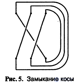
It is easy to see that by closing a braid, i.e., connecting in the simplest
way Ai with Bi, i = 1,..., n, as shown in Fig. 5, we obtain a
diagram of a knot or link.
The book describes three important theorems related to braids.
Alexander's theorem (see, for example, [123]) states that every
isotopy class of a knot or link can be obtained as the
closure of a braid; Artin's theorem (see [5]) gives a presentation of braid groups
by generators and relations; and Markov's theorem [66] describes
the moves on braids that leave the isotopy class of the knot unchanged.
Dehornoy's algorithm, which recognizes the isotopy of braids, is also based on Markov's theorem;
a separate lecture will be devoted to this algorithm.
A notable advantage of braid theory is that it is
algebraic, i.e., every knot can be written as a word (generally
speaking, in an infinite alphabet).
Of the literature covering everything described above, I recommend
the two books by Louis Kauffman [47, 48], as well as the books by C. Adams [1],
A. Kawauchi [52], and (in Russian) [94].
Suppose we have a knot and want to change its
isotopy class by smoothly changing the map of the circle into R3. This cannot be done without
an intersection, so the moment of
intersection is the most important. If in such a map there is exactly
one intersection, exactly two branches of the knot take part in it, and they intersect
transversally, then such a map of the circle into R3 is called a singular
knot. The space of singular knots is called the discriminant
space.
Studying the properties of discriminants, V. A. Vassiliev introduced the notion of
finite-type invariants, which subsequently became known as
Vassiliev invariants. Initially, Vassiliev invariants required
a large amount of non-elementary mathematical machinery, but
later a simple combinatorial interpretation of them was found, which
will be described later. It will also be proved below that
Vassiliev invariants are stronger than all the polynomial
invariants listed above.
The proof of the existence of Vassiliev invariants originally
appeared in [85]; the structure of these invariants (for knots only)
was obtained by M. L. Kontsevich by means of a remarkable
construction, the famous integral that bears his name. In the first versions of
Kontsevich's work (before publication) an error was found, which D. Bar-Natan
reported to him, after which Kontsevich corrected his work. This
work can be read in [56]. We also suggest studying the
construction of the Kontsevich integral from the paper [13]. In [13] the algebras of
chord diagrams and Chinese character diagrams are studied, as well as their relation to invariants of
representations of Lie algebras.
For a long time, computing the Kontsevich integral was very
difficult until the paper of Le and Murakami [63] appeared, in which
they essentially present a technique for such a computation. It is,
however, quite complicated, and we will not deal with it.
There is one more beautiful way of representing all knots and
links; it is based on the notion of a d-diagram introduced in [107],
a circle with two families of disjoint chords; d-diagrams
are the subject of the fourth chapter of this book. This theory originates
from the theory of atoms and Hamiltonian systems and makes it possible to construct a
bracket semigroup of knots, thereby describing all knots and links
as words in a finite alphabet of four letters, see [107]. This is
the advantage of encoding by means of d-diagrams, for example,
over encoding by means of braids, which requires an infinite set of
letters. Moreover, this approach generalizes simply and elegantly to the case of
singular knots, which makes it possible to describe Vassiliev invariants
as words in a finite alphabet.
By means of d-diagrams, all knots and links are represented
as loops on graph paper, starting at the origin
and lying inside the first quadrant.
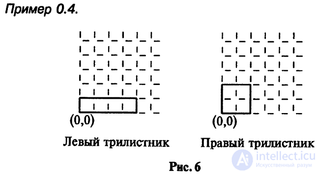
The left trefoil can be written as a 1x4 rectangle, the right one
as a 2x2 square, see Fig. 6.
In general, the theory of atoms, originally invented for
the classification of Hamiltonian systems, turns out to be applicable in
many areas of geometry and topology, for example, for encoding 3-
manifolds.
Finally, I will mention the notion of a virtual knot introduced by Louis Kauffman in 1996,
a combinatorial notion based on the
knot diagram. The theory of virtual knots can be interpreted
as a "projection" of knot theory in various three-dimensional
manifolds. This theory is developing rapidly and has much in common in its approaches
with classical knot theory.
Knots have been used everywhere since antiquity. This is explained by their important technological role, especially in seafaring and construction. But ropes and knots appeared earlier, in prehistoric times, and preceded the invention of the axe, the bow, and the wheel. Today we use knots without even thinking that their age is measured in millennia. It does not even occur to us that knots such as the clove hitch, the reef knot, and the bowline (see Fig. 0.1) served the inhabitants of Ancient Egypt five thousand years ago. (For example, a clove hitch was found on the door of the third chamber of the tomb of the pharaoh Tutankhamun.)
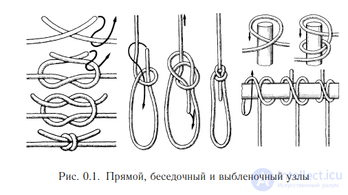
The reef (or square) knot, well known in Ancient Egypt, was widespread in the everyday life of the ancient Greeks and Romans. It adorned the staff of the ancient Roman god Mercury, the patron of trade, and was called nodus Hercules, the Herculean knot, because this ancient hero wore the skin of a slain lion, whose front paws he tied on his chest in exactly this way.
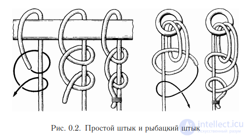
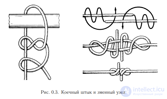
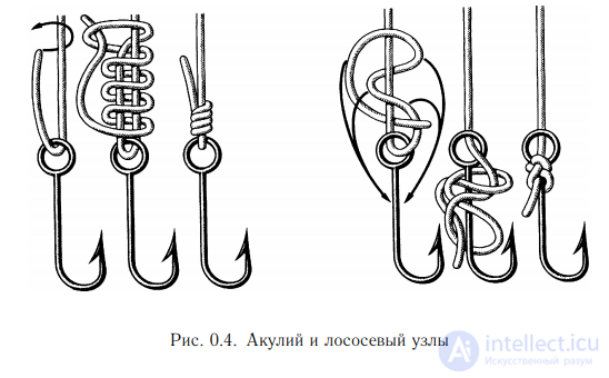
Sailors turned out to be the inventors of the most ingenious and reliable knots. After all, it was they, more often than permanent dwellers on land, who had to deal with ropes and cables. The best of the knots have survived for centuries, passing from generation to generation (see Adams, 1994, which gives pictures of more than 700 different knots). Here we will consider only a few examples of knots. Thus, the simple bowline is used for hoisting loads; the fisherman's bend (or anchor knot) is recognized by sailors of all countries as the most reliable for attaching a rope to an anchor (Fig. 0.2). The hammock bowline is used for fastening hanging hammocks on ships; a snake knot (sheet bend) can firmly tie together two fishing lines (Fig. 0.3). Figure 0.4 shows two of the many fishing knots: the shark knot and the salmon knot.
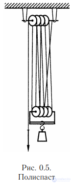
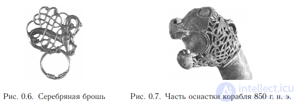
One of the first authors of writings about knots was the Englishman John Smith, known to every American schoolchild for his romantic adventures with the beautiful Native American princess Pocahontas, which ended so tragically for her. In 1627 he published a nautical dictionary in which he described some knots. A century later knots became the subject of a detailed article in the "Encyclopédie" of Diderot and d'Alembert. Many special knots are connected with one of the principal technological inventions of antiquity, the pulley block. Figure 0.5 shows a block and tackle, a sort of rope lever of Archimedes. This device combines two great inventions, the wheel and the rope, and is used for hoisting loads. Along with technological and practical applications, one should certainly also mention the aesthetic and magical aspects. The Scandinavian peoples (possibly because of their inseparable connection with the sea) were especially fond of decorations in the form of knots (Fig. 0.6). They were often placed on weapons and on the stems of ships (Fig. 0.7), and used to create patterns
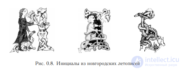
One of the most striking uses of knots can be seen in the ornaments of Bulgarian, Novgorod, and Moscow chronicles of the 12th–14th centuries (Fig. 0.8).
Today we find ourselves in a position close to that of 1860: many researchers believe, as William Thomson did in his day, that knots play a key role in the fundamental physical theory describing the structure of matter. However, this is not a return to the starting point: the spiral of knowledge has made a full turn, and we find ourselves in the same position, but at a higher level.
Knot theory remains alive and enigmatic. The main problems are still open: knots continue to elude attempts to classify them clearly, and it is still unknown whether they possess an easily computable complete system of invariants. And finally, the fundamental role that they are believed to play in physics has still not been fully determined

Comments