
Lecture 7 min.
This lecture is about knots, their planar
diagrams and Reidemeister moves, as well as the semigroup
structure on the set of knots, which is isomorphic to the semigroup structure
on the semigroup of natural numbers under multiplication. Such a similarity of
structures on the set of knots and the set of natural numbers gives grounds
to speak of the arithmetic of knots. Many examples will also be given.
Although the accompanying material on geometry and topology
will be presented within this special course, the audience is encouraged
to become familiar with the basic definitions, for example, in [126]. The reader can
become acquainted with some illustrative topological constructions
in [122].
Since a knot is a smooth embedding of a circle
into R3, it can be approximated arbitrarily closely
by an embedding of a closed polygonal line into R3, without leaving its isotopy
class.
Definition 1.1. An embedding of a closed polygonal line into R3 is called
a polygonal knot.
Definition 1.2. A knot (link) is called tame if it is
isotopic to a polygonal knot (link); otherwise the
knot (link) is called wild.
Remark 1.1. The distinction between tame and wild knots is of
paramount importance. Almost all statements of this book apply
only to tame knots. All C1-smooth knots are tame;
for a proof see [104]. In what follows we will assume all knots to be smooth and,
consequently, tame, unless stated otherwise.
Exercise 1.1. Define a polygonal link carefully.
Definition 1.3. We say that two polygonal knots
(links) are isotopic if one of them can be transformed into the other by
a multiple composition of the so-called elementary
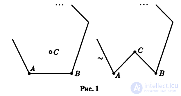
isotopy, which consists in replacing an edge AB of a closed polygonal line by two
edges AC and BC, provided that the triangle ABC does not intersect
other edges of the closed polygonal line of the given knot, as well as of the transformation inverse
to the elementary isotopy, see Fig. 1.
For polygonal knots, as for smooth ones, one can
consider planar diagrams with overpasses and underpasses, and from the graph
with overpasses and underpasses one can recover the polygonal knot
up to isotopy; in particular, for a sufficiently good
approximation of a smooth knot by a polygonal one, the planar diagram will
have the same combinatorial structure.
Exercise 1.2. Show that all polygonal knots with fewer than
six edges are trivial.
Exercise 1.3. Give an example of a polygonal trefoil with
six edges.
Definition 1.4. A planar isotopy of a planar
diagram of a smooth knot (link) is a homeomorphism of the plane onto itself
that does not change the combinatorial structure of the 2-complex
obtained by dividing the plane into cells by the projection graph of the knot, and
preserves the structure of overpasses and underpasses at the vertices of the projection.
Remark 1.2. A planar isotopy of a polygonal
knot, defined analogously, should not be sensitive to bivalent vertices; thus, by splitting an
edge into two by an additional vertex, we obtain a diagram that is
planar-isotopic to the original.
Remark 1.3. A planar isotopy does not change the isotopy class of a knot
in the space R3.
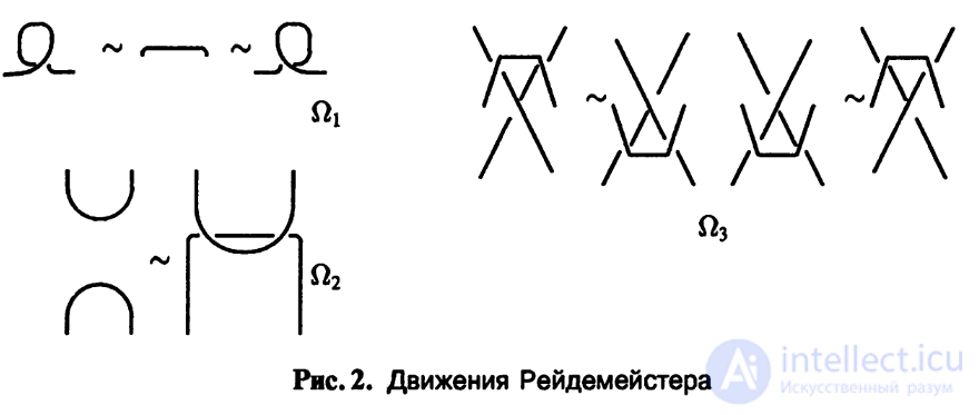
Theorem 1.1 (Reidemeister, [79]). Two planar diagrams D1 and D2
of smooth knots (links) give isotopic knots (links)
if and only if D1 can be transformed into D2 by
a sequence of planar isotopies and the three Reidemeister moves
 see Fig. 2.
One proof of this theorem is based on the notion of
codimension; here we give another proof, based
on the use of polygonal knots (links).
Proof. In one direction the proof is obvious. It suffices only
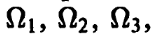
to check that all the moves Ω1, Ω2, Ω3 do not change the
isotopy class of the knot.
Let us prove the statement of the theorem in the converse direction. So, let
two isotopic knots K1 and K2 be given by their planar
diagrams D1 and D2 with overpasses and underpasses. Then there exists a continuous
isotopy of the knot K1 to the knot K2 in the space R3. We approximate these
knots by polygonal knots K'1 and K'2 and consider an isotopy from K'1
to K'2 consisting of elementary isotopies [AB] → [AC]∪[CB].
Without loss of generality we may assume that at each step, for the
corresponding triangle ABC, the edges [DA] and [BE] emerging
from the endpoints of the segment [AB] do not intersect the interior of the
triangle ABC. Otherwise this can easily be achieved by means of
the move Ω1.
It is easy to see that the components of the intersection of the projection of the triangle
ABC with L0, where L0 is the projection of the given link onto the plane ABC,
are of upper and lower kinds, i.e., the corresponding branches of the link L
lie below (or above) the plane ABC.
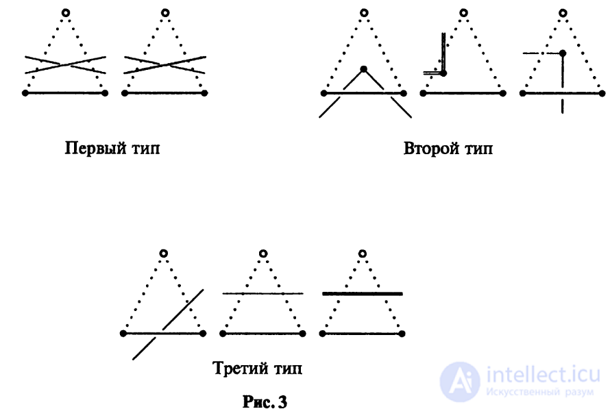
Let us divide the triangle ABC into small triangles of four
types, whose sides do not contain vertices of the projection L0 (see Fig. 3).
A triangle of the first type contains exactly one crossing of L0, and
the branches of L0 intersect exactly two sides of this triangle.
A triangle of the second type contains exactly one vertex of L0 and parts of the
edges emerging from it. A triangle of the third type contains part of
exactly one edge of L0 and contains no vertices. Finally, a triangle
of the fourth type contains neither vertices nor edges (it is not
shown in Fig. 3).
Such a triangulation of the triangle ABC can be constructed
as follows. First, for each crossing and each vertex
we construct triangles of the first and second types, and then we cut
the remaining part of the triangle ABC into triangles of the third and fourth
types.
Now, instead of the original elementary transformation of
the triangle ABC, we will perform elementary transformations of four
types for the small triangles. Figure 3 shows that the move for
a triangle of the first type corresponds to a combination of the third and second
Reidemeister moves Ω3, Ω2; for triangles of the second or
third type, to Ω1, Ω2 or a planar isotopy. The move for a triangle of the
fourth type is a planar isotopy.
Thus the theorem is proved. ■
Exercise 1.4. Show that the two variants of the third Reidemeister
move shown in Fig. 2 are dependent, i.e., either of them is derived from
the other together with the second Reidemeister move.
At the same time, all three Reidemeister moves Ω1, Ω2, Ω3 are
independent of each other. Their independence will be shown in
Appendix 1.
Definition 1.5. A knot is called invertible if it is isotopic to
the knot obtained from it by reversing the orientation.
Remark 1.4. One should not confuse the invertibility of a knot with its having
an inverse (in the sense of composition, see Def. 1.6).
Exercise 1.5. Using Reidemeister moves, show that the
right and left trefoils are invertible knots.
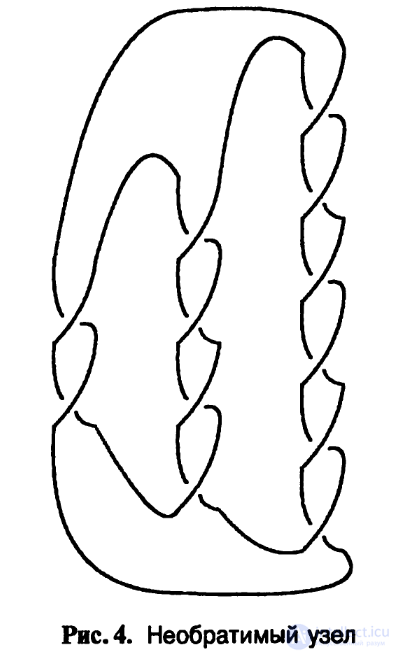
The existence of non-invertible knots was a problem for a long time.
It was solved only in 1964, see [82].
An example of a non-invertible knot is shown in Fig. 4.

Comments