The Derivative. Table of Derivatives. Physical Applications of the Derivative

Concept of the derivative.

Let be defined at the point and in some neighbourhood of it.

Let be a point of the neighbourhood under consideration; then the increment of the argument at the point is called the value 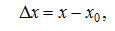, and the increment of the function – the value . If we express , then .

The derivative of the function at the point is called the limit of the ratio of the increment of the function to the increment of the argument, as the latter tends to zero, provided that the limit exists.

The derivative at a point is denoted by . By definition

, (1)

or, equivalently,

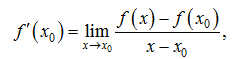, (2)

provided that the limits (1),(2) exist.

A function that has a derivative at a point is called differentiable at that point. The operation of finding the derivative is called differentiation.

The derivative of a function at a point is a number. If a function is differentiable on some set X within its domain of definition, then is also a function (it is also denoted by ).

Basic rules of differentiation

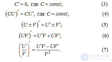
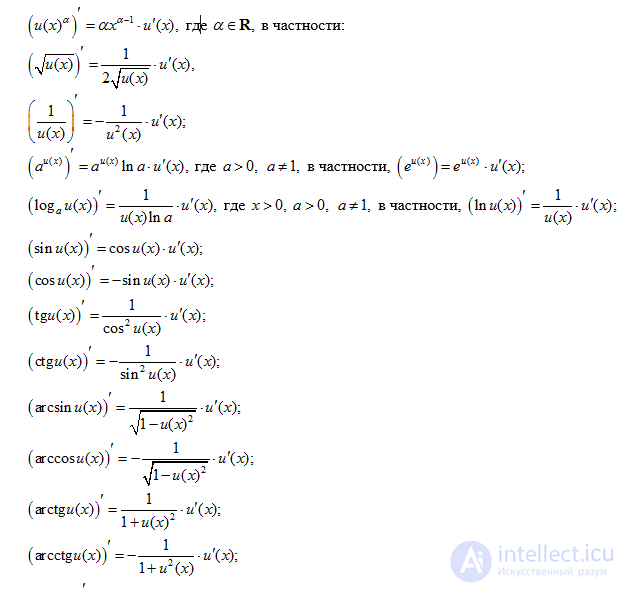
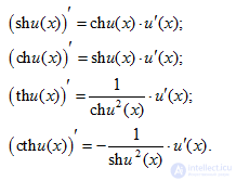
Let be differentiable functions. The following formulas hold:

Derivative of a composite function

If and – are differentiable functions of their arguments, then the derivative of the composite function

is calculated by the formula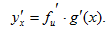

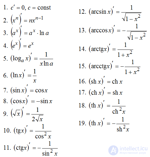
Some applications of the derivative

Table of derivatives.

derivative of sine, cosine, tangent, arctangent, logarithm, constant

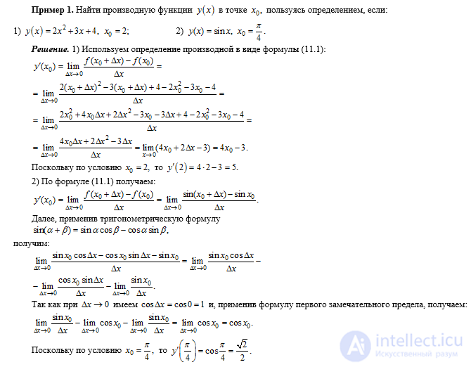
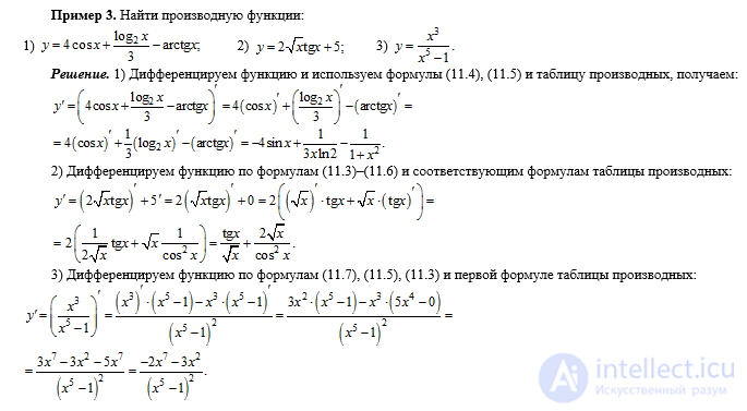
Example

Generalized table of derivatives

If for the function there exists an inverse function ,

which has a derivative then the formula 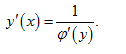holds

Physical application of the derivative . application of the derivative in practice

Equation of the tangent line and the normal

The derivative of the function at the point represents the slope of the tangent line drawn to the graph of the function at the point

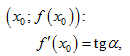
where – is the angle of inclination of the tangent line to the axis Ox. This is the essence of the geometric meaning of the derivative.

The equation of the tangent line drawn to the graph of the function at the point has the form:

(11.9)

The straight line passing through the point of the graph of the function perpendicular to the tangent line drawn at that point,

is called the normal to the graph of the function at the point (Fig. 11.1).

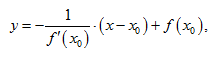
The equation of the normal has the form:

(11.10)

where

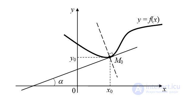
Fig. 11.1

Physical application of the derivative

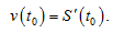
1. KINEMATICS If a material point M moves non-uniformly along a path given by the function then the instantaneous velocity of motion at the moment of time is the derivative of the distance S with respect to time t: (11.11)

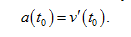
2.KINEMATICS If the function describes the process of change of velocity of non-uniform motion as a function of time, then the instantaneous acceleration of a material point at the moment of time is the derivative of the velocity v with respect to time t: (11.12)

3.THERMODYNAMICS If – is a function describing the process of change of the amount of heat supplied to a body when it is heated to temperature T, then the heat capacity of the body is the derivative of the amount of heat Q with respect to temperature T: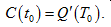

4. MATERIALS SCIENCE Linear density of a non-uniform thin rod at the point is the derivative of the mass m with respect to length l: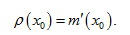

5. ELECTRODYNAMICS The instantaneous value of the electromotive force of induction is equal to the rate of change of the magnetic flux ,

i.e. the derivative of the magnetic flux with respect to time t:

6. The electric current in an oscillating circuit at the moment of time is equal to the derivative of the charge q with respect to time t:

7. Maximum power of the current.

The power of the current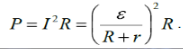

It is known that a function has an extremum (max or min) at a point at which its derivative equals zero. In this case

From the solution of the resulting equation it follows that the maximum power at the load can be achieved if its resistance R equals the internal
resistance of the current source r. That is,

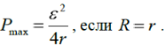
8. Instantaneous value of the alternating current

For example, in electromagnetic oscillations arising in an oscillating circuit, the charge on the plates of the capacitor changes

according to the law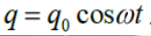

then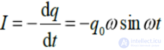

Example 1. Write the equation of the tangent line and the normal drawn to the graph of the function at the point with abscissa x = 2.

Solution.To find the equation of the tangent line we use formula (9). First let us find the ordinate of the point of tangency

. For this, substitute the value x=2 into the equation of the function:

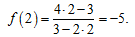
To find the slope we find the derivative , using the formula for differentiating a fraction:

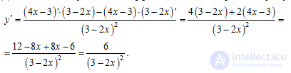
Let us find the value of the derivative at x=2 :

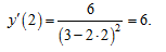
Substituting the values found into formula (9), we obtain the equation of the tangent line:

To write the equation of the normal, we use formula (10):

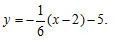
We obtain that the equation of the normal drawn to the given curve at the given point has the form

Example 2. Determine at which point of the curve the tangent line is inclined to the x-axis at an angle of 45°.

Solution. Since the tangent of the angle of inclination of the tangent line to the x-axis equals the value of the derivative at the point of tangency, let us find the derivative of the function:

.

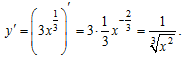By condition Hence, .

From this

, , .

We obtained two values of the abscissa of the point of tangency:

, ,

i.e. there exist two points of tangency at which the tangent line forms an angle with the axis .

Let us find the corresponding ordinates of the points of tangency, substituting the values into the formula of the function:

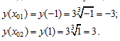
We arrive at the answer: at the points and the tangent line to the given curve forms with the axis the angle

Example 3. Find the acute angle between the parabolas and at the point of their intersection having a negative abscissa.

Solution. The angle between two curves at their point of intersection - is the angle between the tangent lines to these curves drawn at the point of their intersection. The tangent of this angle is calculated by the formula:

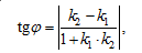(13)

where and -are the slopes of the given parabolas.

Let us find the point of intersection of these parabolas. For this we solve the system:

From this The condition of the problem is satisfied by the point Let us find the coefficient

Similarly, let us find :

Let us use the formula and obtain:

,

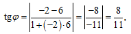whence

Example 4. A body moves in a straight line according to the law Find the velocity of motion of the body at the moment when the acceleration equals zero.

Solution. According to formula (11) the velocity is the derivative of the distance, and, according to formula (12), the acceleration is the derivative of the velocity.

Let us successively compute the derivatives:

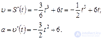
Let us find the moment of time when the acceleration equals zero:

Let us compute the velocity of motion of the body at the moment of time

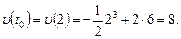
example problem physics - heat

Calculate the amount of heat required to heat 1 kg of a substance from 0 degrees to t degrees (Celsius).

solution

Let Q=Q(t). Consider a small segment [t; t+Δt], on this segment

ΔQ=c(t) • Δt

c(t)= ΔQ/Δt

As Δt→0 lim ΔQ/Δt =Q′(t)

Δt→0

c(t)=Q′(t)

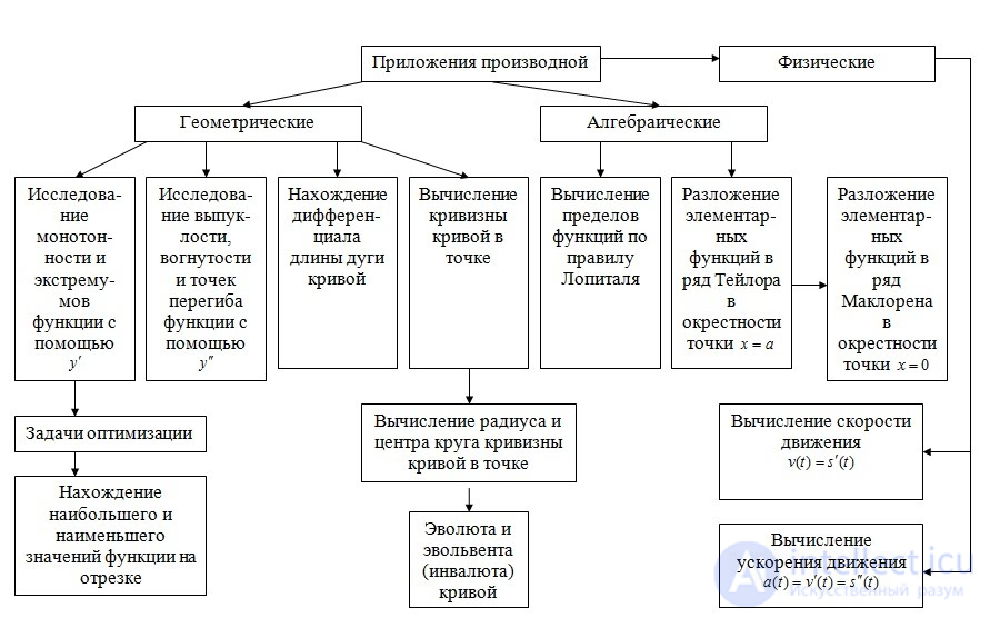
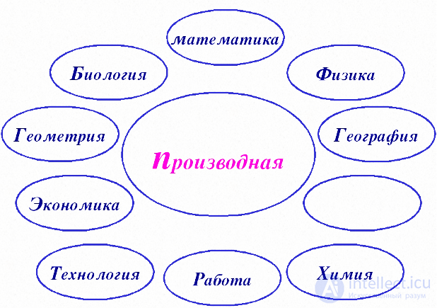
Mathematical modelling is applicable in various fields of knowledge, so the derivative can be used not only in mathematics and disciplines related to it

Application of the derivative in solving applied problems

• Proving inequalities

• Solving equations

• Comparing expressions
• Proving identities
• Solving algebraic and geometric problems

The derivative in chemistry:

Differential calculus has found wide application in chemistry as well, for building mathematical models of chemical reactions and subsequently describing their properties.

The derivative is used in chemistry to determine a very important quantity – the rate of a chemical reaction, one of the decisive factors that must be taken into account in many areas of scientific and industrial activity. V (t) = p ‘(t)

The rate of a chemical reaction in chemistry is the change in the concentration of the reacting substances per unit time, or the derivative of the concentration of the reacting substances with respect to time (in the language of mathematics the concentration would be the function, and time – the argument)

example

Let the amount of substance that has entered into the chemical reaction be given by the relationship: p(t) = t2/2 + 3t –3 (mol)

Find the rate of the chemical reaction after 3 seconds.

solution

p(t) = t2/2 + 3t –3 (mol)

1. Let us find the derivative of the function: P’(t) = t +3

2. Substitute the value t = 3 sec: P’(3) = 3 + 3 = 6 (mol/sec )

Answer: 6 (mol/sec )

The derivative in biology:

A population is a totality of individuals of a given species occupying a defined area of territory within the species’ range, freely interbreeding with one another and partially or fully isolated from other populations, and is also an elementary unit of evolution.

Concept in the language of biology	Notation	Concept in the language of mathematics
Population size at time t1	x = x(t)	Function
Time interval	∆t = t2 – t1	Increment of the argument
Change in population size	∆x = x(t2) – x(t1)	Increment of the function
Rate of change of population size	x = x‘ (t) =∆x/∆t	Ratio of the increment of the function to the increment of the argument
Relative growth at the given moment	∆x/∆t	Derivative

The derivative in geography:

The derivative helps to calculate:

1. Certain values in seismography

of greatest importance for seismogeodynamics are the derivatives of the velocities of movement of the earth’s crust, the most important of which is the gradient, characterizing the rate of deformation. For the field of the vertical component of velocity, maps of the gradient modulus were compiled at the time [Gzovsky, 1967; Nikolaev, Shenkareva, 1967].

2. Features of the earth’s electromagnetic field

Higher derivatives were not only used in the interpretation of potential fields, but also contributed to the development of several new directions in the geological interpretation of observed anomalies: 1) localization of singular points of potential functions; 2) separation of complex anomalies caused by rocks occurring at different depths; 3) attenuation of regional influence; 4) study of the figure of the Earth; 5) solution of problems of reduction of gravitational observations, etc.

3. Radioactivity of geophysical nuclear indicators

4.Many values in economic geography

5.Derive a formula for calculating the population size in a territory at time t.

y’= k y

The idea of the sociological model of Thomas Malthus is that population growth is proportional to the size of the population at the given time t through N(t) .Malthus’s model worked fairly well for describing the population of the USA from 1790 to 1860. Today this model does not hold in most countries

Let us derive a formula for calculating the population size in a limited territory at time t.

Let y = y(t) be the population size.

Let us consider the population growth over Δt = t-t0

Δy = k y Δt, where k = kr – ks – the growth rate coefficient (kr is the birth rate coefficient, ks is the death rate coefficient)

Δy:Δt=k y

As Δt→0 we obtain lim Δy/ Δt=y’.

The derivative in electrical engineering:

In our homes, in transport, in factories: everywhere electric current is at work. By electric current is meant the directed motion of free electrically charged particles.

The quantitative characteristic of electric current is the current strength.

In an electric circuit the electric charge changes with time according to the law q=q (t). The current strength I is the derivative of the charge q with respect to time.

In electrical engineering the operation of alternating current is mainly used.

Electric current that changes over time is called alternating current. An alternating current circuit may contain various elements: heating devices, coils, capacitors.

The generation of alternating electric current is based on the law of electromagnetic induction, the formulation of which contains the derivative of the magnetic flux.

The derivative in economics:

Economics is the basis of life, and within it an important place is occupied by differential calculus – an apparatus for economic analysis. The basic task of economic analysis is the study of the relationships between economic quantities in the form of functions.

The derivative in economics solves important questions:

1. In which direction will state revenue change when taxes are increased or customs duties are introduced?

2. Will a firm’s revenue increase or decrease when the price of its output is increased?

To answer these questions one needs to construct functions relating the variables involved, which are then studied by the methods of differential calculus.

Also, with the help of the extremum of a function (the derivative) in economics one can find the highest labour productivity, maximum profit, maximum output and minimum costs.

Let us consider a situation: let y be the cost of production, and x be the quantity of output, then x1 is the increment of output, and y1 is the increment of the production costs.

In this case the derivative expresses the marginal cost of production and approximately characterizes the additional expenditure on producing an additional unit of output.

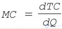
Where:

MC - marginal costs;

TC - total costs;

Q - quantity.

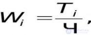
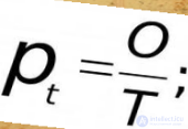
Labour productivity

The derivative can also be used to determine labour productivity:

Let the function u = u(t) express the quantity of output produced u over time t. It is necessary to find the labour productivity at the moment tο.

Over the period of time from tο to tο + Δt the quantity of output produced changes from the value uο = u(tο) to the value uο +Δu = u(tο + Δt). Then

the average labour productivity over this period of time is Zav =Δu :Δt. Clearly, the labour productivity at the moment tο
can be defined as the limiting value of the average productivity over the period of time from tο to tο + Δt as Δt→ 0, i.e.

z = lim Zav = lim Δu/Δt = u'(t) as Δt→0

Problem in economic theory.

An enterprise produces X units of a certain homogeneous output per month. It has been established that the dependence of the enterprise’s financial accumulation on the volume of output is expressed by the formula f(x)=-0,02x^3+600x -1000. Investigate the potential of the enterprise.

The function is investigated by means of the derivative. We obtain that at X=100 the function reaches a maximum.

Conclusion: the enterprise’s financial accumulation grows as the volume of production increases up to 100 units; at x =100 it reaches its maximum and the amount of accumulation equals 39000 monetary units. Further growth of production leads to a reduction in financial accumulation.

Thus , problems solved with the help of the derivative are widely used in production.

CONCLUSION: the derivative is successfully applied in solving various applied problems in science, technology and life

As is evident from the above, the application of the derivative of a function is very diverse and not only in the study of mathematics, but of other disciplines as well. Therefore it can be concluded that the study of the topic: «The derivative of a function» will find its application in other topics and subjects.