
Lecture
A differential equation — is an equation that includes derivatives of a function, and may also include the function itself, the independent variable and parameters. The order of the derivatives occurring in the equation may vary (formally, it is not limited in any way). Derivatives, functions, independent variables and parameters may occur in the equation in various combinations, or may be absent altogether, except for at least one derivative. Not every equation containing derivatives of an unknown function is a differential equation. For example,  is not a differential equation
Unlike algebraic equations, whose solution yields a number (or several numbers), solving a differential equation yields a function (a family of functions).
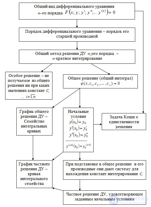
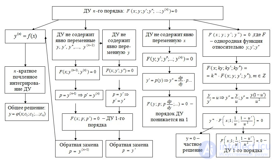
A differential equation of order higher than the first can be transformed into a system of first-order equations, in which the number of equations equals the order of the original differential equation.
Modern high-speed computers efficiently provide a numerical solution of ordinary differential equations, without requiring the solution to be obtained in analytical form. This has allowed some researchers to assert that a problem is considered solved once it has been reduced to the solution of an ordinary differential equation.
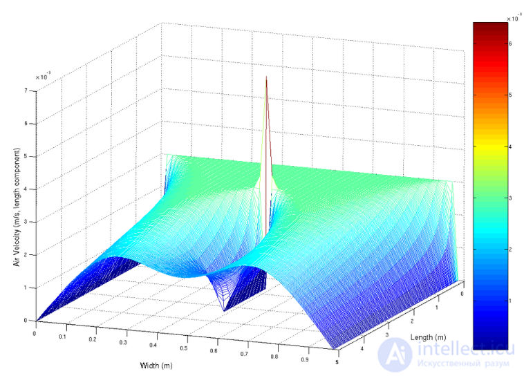
Visualization of airflow computed by solving the Navier-Stokes equation
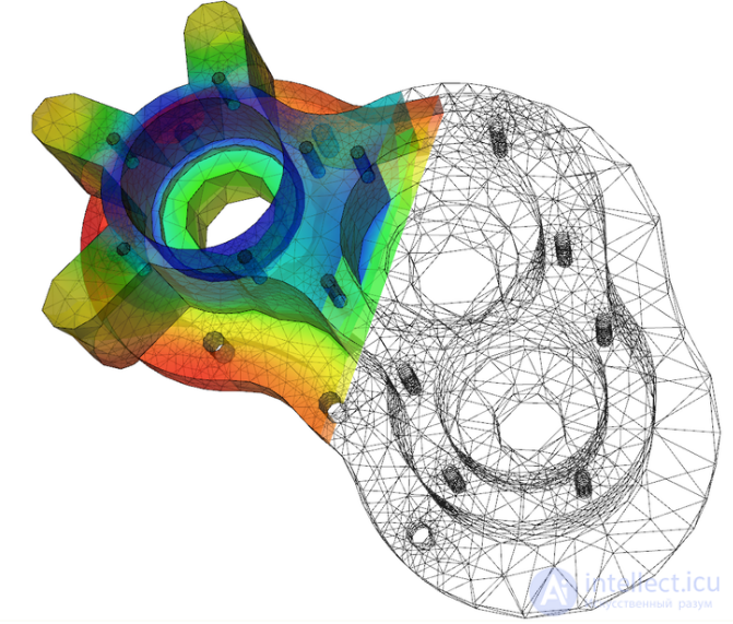
Visualization of heat transfer in a pump housing, obtained by solving the heat conduction equation
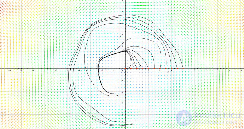
The order of a differential equation — is the highest order of the derivatives appearing in it.
If a differential equation is a polynomial with respect to the highest derivative, then the degree of this polynomial is called the degree of the differential equation. Thus, for example, the equation  is an equation of the second order, of the fourth degree .
The solution (integral) of a differential equation of order n is a function y(x), having on some interval (a, b) derivatives  up to order n inclusive and satisfying this equation. The process of solving a differential equation is called integration. The problem of integrating a differential equation is considered solved if finding the unknown function
  can be reduced to quadrature, (i. e. to the form
 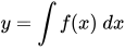 , where
  — is an elementary function) regardless of whether the resulting integral is expressed in closed form through known functions or not.
All differential equations can be divided into ordinary (ODEs), which involve only functions (and their derivatives) of a single argument, and partial differential equations (PDEs), in which the functions involved depend on several variables. There also exist stochastic differential equations (SDEs), which involve random processes.
Depending on the combinations of derivatives, functions and independent variables, differential equations are classified as linear and nonlinear, with constant or variable coefficients, homogeneous or inhomogeneous. Because of the importance of their applications, quasilinear (linear with respect to the highest derivatives) partial differential equations are singled out as a separate class .
The most important question for differential equations is the existence and uniqueness of their solution. This question is resolved by existence and uniqueness theorems, which state the necessary and sufficient conditions for it. For ordinary differential equations, such conditions were formulated by Lipschitz (1864). For partial differential equations, the corresponding theorem was proved by S. V. Kovalevskaya (1874).
Solutions of differential equations are divided into general and particular solutions. General solutions include undetermined constants, and, for partial differential equations, — arbitrary functions of the independent variables, which can be specified from additional conditions of integration (initial conditions for ordinary differential equations, initial and boundary conditions for partial differential equations). Once the form of these constants and undetermined functions has been determined, the solutions become particular.
The search for solutions of ordinary differential equations led to the establishment of a class of special functions — functions that often occur in applications and cannot be expressed through known elementary functions. Their properties have been studied in detail, tables of values have been compiled, mutual relationships have been established, and so on.
The development of the theory of differential equations has, in a number of cases, made it possible to dispense with the requirement of continuity of the functions under study and to introduce generalized solutions of differential equations.
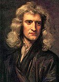
Isaac Newton
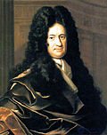
Gottfried Leibniz

Leonhard Euler
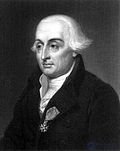
Joseph-Louis Lagrange
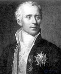
Pierre-Simon Laplace
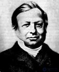
Joseph Liouville
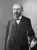
Henri Poincaré
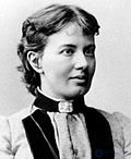
Sofya Kovalevskaya
Originally, differential equations arose from problems of mechanics, in which it was necessary to determine the coordinates of bodies, their velocities and accelerations, considered as functions of time under various actions. Certain geometric problems considered at that time also led to differential equations.
The foundation of the theory of differential equations was differential calculus, created by Leibniz and Newton (1642—1727). The term «differential equation» itself was proposed in 1676 by Leibniz.
Among the huge number of eighteenth-century works on differential equations, the works of Euler (1707—1783) and Lagrange (1736—1813) stand out. In these works, the theory of small oscillations was first developed, and consequently — the theory of linear systems of differential equations; along the way, the basic concepts of linear algebra arose (eigenvalues and eigenvectors in the n-dimensional case). Following Newton, Laplace and Lagrange, and later Gauss (1777—1855), also developed methods of perturbation theory.
When the unsolvability of algebraic equations in radicals had been proved, Joseph Liouville (1809—1882) constructed an analogous theory for differential equations, establishing the impossibility of solving a number of equations (in particular such classical ones as linear second-order equations) in elementary functions and quadrature. Later, Sophus Lie (1842—1899), analysing the question of integrating equations in quadratures, came to the necessity of studying in detail groups of diffeomorphisms (subsequently named Lie groups) — thus, from the theory of differential equations, arose one of the most fruitful areas of modern mathematics, whose further development was closely connected with entirely different questions (Lie algebras had already been considered earlier by Siméon Denis Poisson (1781—1840) and, especially, by Carl Gustav Jacob Jacobi (1804—1851)).
A new stage in the development of the theory of differential equations begins with the works of Henri Poincaré (1854—1912); the «qualitative theory of differential equations» that he created, together with the theory of functions of complex variables, formed the basis of modern topology. The qualitative theory of differential equations, or, as it is now more often called, the theory of dynamical systems, is currently developing actively and has important applications in the natural sciences.
Ordinary differential equations (ODEs) — are equations that depend on a single independent variable; they have the form
 or
or 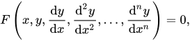
where  — is an unknown function (possibly a vector function; in that case one often speaks of a system of differential equations), depending on the independent variable {\displaystyle x,}
 the prime denotes differentiation with respect to
  The number
  is called the order of the differential equation. The most practically important are differential equations of the first and second order.
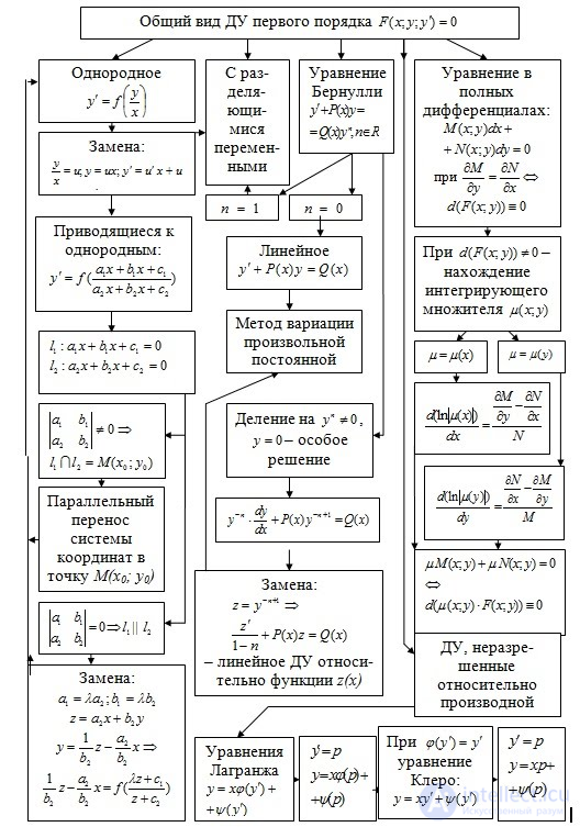
The simplest first-order differential equations — are a class of first-order differential equations that are the easiest to solve and study. This class includes equations in total differentials, equations with separable variables, homogeneous first-order equations and linear first-order equations. All these equations can be integrated in closed form.
The starting point of the exposition will be a first-order differential equation, written in the so-called symmetric form:

where the functions  and
and  are defined and continuous in some domain
  .
.
Partial differential equations (PDEs) — are equations containing unknown functions of several variables and their partial derivatives. The general form of such equations can be represented as:

where {\displaystyle x_{1},x_{2},\dots ,x_{m}} — are the independent variables, and
  — is a function of these variables. The order of a partial differential equation can be defined in the same way as for ordinary differential equations. Another important classification of partial differential equations is their division into equations of elliptic, parabolic and hyperbolic type, especially for second-order equations.
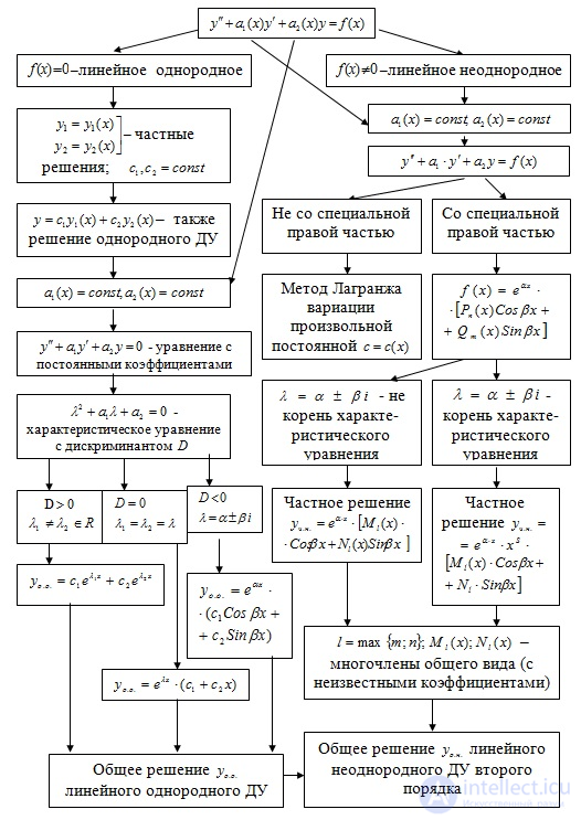
Both ordinary differential equations and partial differential equations can be divided into linear and nonlinear ones. A differential equation is linear if the unknown function and its derivatives enter the equation only to the first power (and are not multiplied by one another). For such equations the solutions form an affine subspace of the space of functions. The theory of linear ODEs is developed considerably more deeply than the theory of nonlinear equations. The general form of a linear differential equation of order n:

where pi(x) — are known functions of the independent variable, called the coefficients of the equation. The function r(x) on the right-hand side is called the free term (the only term that does not depend on the unknown function). An important special class of linear equations is linear differential equations with constant coefficients.
A subclass of linear equations is formed by homogeneous differential equations — equations that contain no free term: r(x) = 0. For homogeneous differential equations the superposition principle holds: a linear combination of particular solutions of such an equation is also a solution of it. All other linear differential equations are called inhomogeneous differential equations.
Nonlinear differential equations in the general case have no developed methods of solution, except for some special classes. In some cases (using various approximations) they can be reduced to linear ones. For example, the linear equation of a harmonic oscillator {\displaystyle {\frac 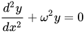 can be regarded as an approximation of the nonlinear equation of a mathematical pendulum
 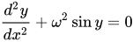 for the case of small amplitudes, when y ≈ sin y.
 — a homogeneous second-order differential equation with constant coefficients. The solution is the family of functions
  , where
  and
and  — are arbitrary constants which, for a specific solution, are determined from separately given initial conditions. This equation, in particular, describes the motion of a harmonic oscillator with cyclic frequency 3.
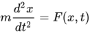
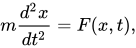 where m — is the mass of the body, x — is its coordinate, F(x, t) — is the force acting on the body with coordinate x at time t. Its solution is the trajectory of the body's motion under the action of the given force.
 Its solutions are the so-called cylindrical functions — the Bessel, Neumann, and Hankel functions.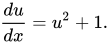
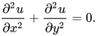
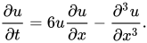
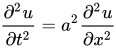
In the following group of examples the unknown function u depends on two variables, x and t, or x and y.
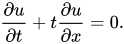
 — is the deflection of the string at the point with coordinate x at time t, and the parameter a sets the properties of the string: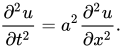
Some differential equations have solutions that can be given by an exact formula. Such classes of equations are presented below.
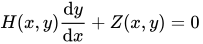
In the table, H ( x ), Z ( x ), H ( y ), Z ( y ) or H ( x , y ), Z ( x , y ) - are arbitrary integrable functions of x or y (or of both parameters ), and A , B , C , I , L , N , M - are constants. In general A , B , C, I , L , are real numbers, while N , M , P and Q may be complex. The differential equations are presented in an alternative form that allows them to be solved by the method of integration.
| differential equations | general solution | |
|---|---|---|
| 1 | 
|
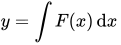 |
| 2 | 
|
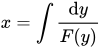 |
| 3 | 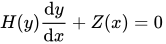
|
 |
| 4 | 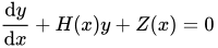
|
 |
| 5 | }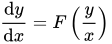 |
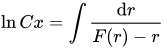
the solution may be an implicit function of x and y , obtained by evaluating the reduced integral using the substitution of variables |
| 6 | 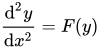 |
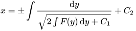 |
|
If the DE is exact, that is 
then the solution is given by the formula: where If the equation is not exact, from the functions H ( x , y ) and Z ( x , y ) an integrating factor can be determined, after multiplying the equation by which it is solved analogously to the exact case. |
|
| 8 | 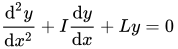 |
if then if then if then |
| 9 | 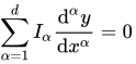 |
where |
Note that 3 and 4 are special cases of 7; they are fairly common and are presented for the sake of completeness.
Equation 8 is also a special case of 9, but 8 is a sufficiently common form of equation, especially in simple physical and engineering problems.
 ,
,
where } - is the mass of the body,
  - is its coordinate,
  - is the force acting on the body with coordinate at time
  . Its solution is the trajectory of the body's motion under the action of the given force.
 ,
,
where - is the deflection of the string at the point with coordinate at time , the parameter  sets the properties of the string.
 :
:  ,
,
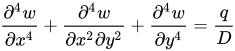
where } - are the vertical deflections of the plate,
  - is the cylindrical stiffness of the plate in bending.
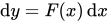
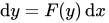





 and
and  - are certain functions, depending on the integrals, that allow the correct determination of the function
  hold.
hold.





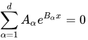
 - are the d roots of a polynomial of degree d :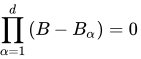

Comments