
Lecture
Perceptual hashing — is the use of a fingerprinting algorithm that produces a snippet, hash, or fingerprint of various forms of media. A perceptual hash is a type of locality-sensitive hash, which is similar if the media's characteristics are similar. This is in contrast to cryptographic hashing, which relies on the avalanche effect, where a small change in the input value causes a drastic change in the output value. Perceptual hash functions are widely used in detecting cases of copyright infringement online, as well as in digital forensics, thanks to the ability to correlate hashes and find similar data (for example, with a different watermark).
Perceptual hashes are a different concept compared to cryptographic hash functions such as MD5 and SHA1. With cryptographic hashes, the resulting values are essentially random. The data used to generate the hash acts as a random seed, so the same data generates the same result, but different data produces different results. Comparing two SHA1 hash values actually only tells you two things. If the hashes are different, the data is different. And if the hashes are the same, the data is most likely the same as well. Perceptual hashes, by contrast, can be compared, giving you a sense of similarity between two sets of data.
Marr and Hildreth's 1980 work is a seminal contribution in this field.
Christoph Zauner's thesis, published in July 2010, is a well-written introduction to the topic.
In June 2016, Azade Amir Asgari published a paper on robust forgery of image hashes. Asgari notes that a perceptual hash function, like any other algorithm, is prone to errors.
In December 2017, researchers noted that Google's image search is based on perceptual hashing.
In a study published in November 2021, investigators focused on a manipulated image of Stacey Abrams that had been posted online before her defeat in the 2018 Georgia gubernatorial election. They found that the pHash algorithm was vulnerable to attackers.
A study published in January 2019 at Northumbria University showed that, for video, it can be used to simultaneously identify similar content for video copy detection and detect malicious manipulation for video authentication. The proposed system performs better than existing video hashing methods, both in terms of identification and authentication.
A study on deep-learning-based perceptual audio hashing, published in May 2020 by the University of Houston, showed better performance than traditional fingerprinting methods for detecting similar/copied audio subjected to transformations.
In addition to its use in digital forensics, a study published in 2019 by a Russian research group showed that perceptual hashing can be applied in a wide variety of situations. Similar to comparing images for copyright infringement, the group found that it can be used to compare and match images in a database. The algorithm they proposed turned out to be not only effective, but also more efficient than standard database image search tools.
In July 2019, a Chinese research group reported that they had found perceptual hashing for speech encryption to be effective. They managed to create a system in which the encryption was not only more accurate, but also more compact.
Back in August 2021, Apple Inc reported on a child sexual abuse material (CSAM) system known as NeuralHash. In a technical summary document that explains the system well with numerous diagrams and sample photos, it states: "Instead of scanning images [on corporate] iCloud [servers], the system performs on-device matching using a database of known CSAM image hashes provided by the [National Center for Missing and Exploited Children] (NCMEC) and other child safety organizations. Apple further transforms this database into an unreadable set of hashes that is securely stored on users' devices".
In an essay titled "The Problem with Perceptual Hashes", Oliver Kuederle describes a striking collision produced by a piece of commercial neural-network software of the NeuralHash type. A portrait photo of a real woman (Adobe Stock) is reduced by the test algorithm to the same hash as a photo of an abstract art piece (from the "deposit photos" database). Both sample images are in commercial databases. Kuederle is concerned about collisions like this. "These cases will be checked by hand. That is, according to Apple, an Apple employee will then look at your (flagged) photos…
Perceptual hashes are messy. When such algorithms are used to detect criminal activity, especially at the scale of large companies, many innocent people could potentially face serious trouble... Needless to say, this worries me a great deal".
Researchers have continued to publish a comprehensive analysis titled "Learning to Break Deep Perceptual Hashing: The Use Case NeuralHash", in which they examine the vulnerability of NeuralHash, as a representative of deep perceptual hashing algorithms, to various attacks. Their results show that hash collisions between different images can be achieved through small changes made to the images. According to the authors, these results demonstrate a real likelihood of such attacks and make it possible to frame and potentially prosecute innocent users. They also state that detection of illegal material can easily be avoided and the system outsmarted using simple image transformations, such as those provided by free image editors. The authors suggest that their findings also apply to other deep perceptual hashing algorithms, calling into question their overall effectiveness and functionality in applications such as client-side scanning and chat moderation.
perceptual hash algorithms describe a class of functions for generating comparable hashes. They use various properties of an image to build an individual "fingerprint". These "fingerprints" can then be compared with one another.
If the hashes differ, the data is different. If the hashes match, the data is most likely the same (since there is a possibility of collisions, matching hashes do not guarantee matching data). This article covers several popular methods for building perceptual image hashes, as well as a simple way to deal with collisions. Anyone interested is welcome to read on.
There are many different approaches to building a perceptual image hash. They all share 3 main stages:
This publication will not cover the implementation of the algorithms described. It is intended as an overview and describes various approaches to building hashes.
Let's look at various hash algorithms: Simple Hash, DCT Based Hash, [11], Radial Variance Based Hash, and Marr-Hildreth Operator Based Hash, .
The essence of this algorithm lies in mapping the average value of the low frequencies. In images, high frequencies provide detail, while low frequencies show structure. Therefore, to build a hash function that produces close hashes for similar images, the high frequencies need to be discarded. How it works:
The resulting hash is robust to scaling, compression or stretching of the image, and changes in brightness, contrast, and color manipulation. But the main advantage of the algorithm is its speed. The normalized Hamming distance function is used to compare hashes of this type.
Original image

Resulting "fingerprint"
The discrete cosine transform (DCT) is one of the orthogonal transforms, closely related to the discrete Fourier transform (DFT) and constituting a homomorphism of its vector space. Like any Fourier-related transform, the DCT expresses a function or signal (a sequence of a finite number of data points) as a sum of sinusoids with different frequencies and amplitudes. The DCT uses only cosine functions, unlike the DFT, which uses both cosine and sine functions. There are 8 types of DCT. The most common is the second type. This is the one we will use to build the hash function.
Let's understand what the second type of DCT is:
Let x[m], where m = 0,…, N — 1 — be a signal sequence of length N. Define the second type of DCT as

This expression can be rewritten as:
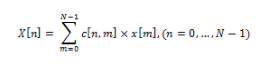
where c[n,m] – is the element of the DCT matrix at the intersection of row n and column m.
The DCT matrix is defined as:
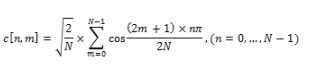
This matrix is very convenient for computing the DCT. The DCT can be precomputed for any required length. Thus the DCT can be represented as:
DCT=M×I×M'
Where M – is the DCT matrix, I – is a square-sized image, M’ – is the inverse matrix.
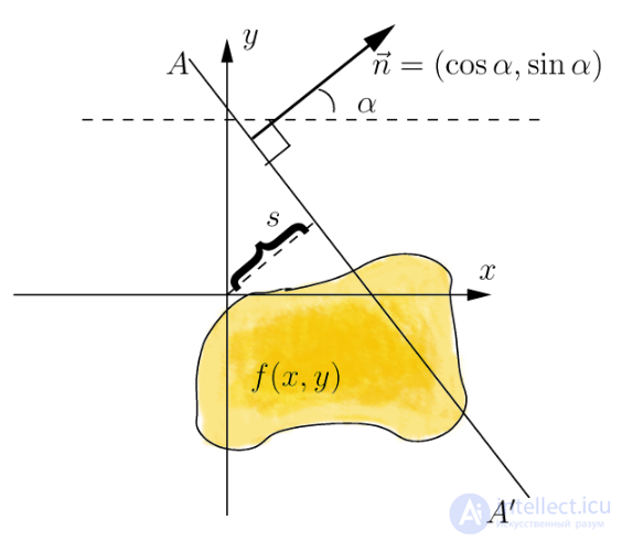
The idea behind the Radial Variance Based Hash algorithm is to build a radial variance vector (RVV) based on the Radon transform. The DCT is then applied to the RVV and the hash is computed. The Radon transform is an integral transform of a function of several variables along a line. It is robust to image processing operations such as compression and geometric transformations such as rotation. In the two-dimensional case, the Radon transform for a function f(x,y) looks like this:
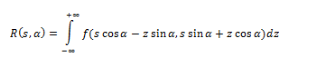
The Radon transform has a simple geometric meaning – it is the integral of the function along a line perpendicular to the vector n = (cos a, sin a) and passing at a distance s (measured along vector n, with the corresponding sign) from the origin.
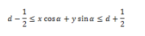
To extend the Radon transform to discrete images, the line integral along the line d = x ∙ cos α + y ∙ sin α can be approximated by summing the values of all pixels lying on a line one pixel wide:
It was later discovered that it is better to use variance instead of the sum of pixel values along the projection line. Variance handles brightness discontinuities along the projection line much better. Such brightness discontinuities appear due to edges that are orthogonal to the projection line.
Now let's define the radial variance vector. Let Γ(α) – be the set of pixels on the projection line corresponding to a given angle. Let (x′, y′) – be the coordinates of the central pixel in the image. x, y belong to Γ(α) if and only if
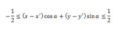
Now let's define the radial variance vector:
Let I(x,y) denote the brightness of pixel (x,y), #Γ(α) – the cardinality of the set, then we define the radial variance vector R[α], where α = 0,1, … ,179 as

It is sufficient to build the vector for 180 angle values, since the Radon transform is symmetric. The resulting vector can be used to build the hash, but this algorithm suggests a further improvement — applying the DCT to the resulting vector. This produces a vector that inherits all the important properties of the DCT. The first 40 coefficients of the resulting vector, which correspond to the low frequencies, are taken as the hash. Thus, the size of the resulting hash is 40 bytes.
The Marr-Hildreth operator makes it possible to detect edges in an image. Generally speaking, a boundary in an image can be defined as an edge or contour separating adjacent parts of the image that have comparatively distinct characteristics according to certain features. These features can be color or texture, but the grayscale value of the image (brightness) is most commonly used. The result of edge detection is an edge map. The edge map describes the edge classification for each pixel of the image. If edges are defined as a sharp change in brightness, derivatives or a gradient can be used to find them.
Let a function denote the brightness level for a line (a one-dimensional array of pixels). The first approach to edge detection consists of finding the local extrema of the function, i.e., the first derivatives. The second approach (the Laplacian method) consists of finding the second derivatives.
Both approaches can be adapted to the case of two-dimensional discrete images, but with some issues. Finding derivatives in the discrete case requires approximation. In addition, noise in the image can significantly degrade the edge-finding process. Therefore, before detecting edges, some noise-suppressing filter must be applied to the image. To build the hash, an algorithm using the Laplace operator (approach 2) and a Gaussian filter can be chosen.
Let's define the continuous Laplacian (Laplace operator):
Let a function define the brightness in the image. Then we define the continuous Laplacian as:

The zero crossings are the points corresponding to the boundary of the function, since these are the points at which the second derivative becomes zero. Various filters (discrete Laplace operators) can be derived from the continuous Laplacian. Such a filter can be applied to a discrete image using convolution of functions. The Laplace operator for an image can be rewritten as:

where * denotes convolution of functions. To build the edge map, we need to find the zero crossings of the discrete operator.
Now let's look at the Marr-Hildreth operator. It is also called the Laplacian of Gaussian (LoG) – a special type of discrete Laplace operator. LoG is constructed by applying the Laplace operator to a Gaussian filter (function). The distinctive feature of this operator is that it can highlight edges at a particular scale. The scale variable can be varied to better reveal edges.
Let's define the Gaussian filter as:

Convolution and the Laplace operation can be swapped, because the derivative and convolution are linear operators:

This property allows the operator to be precomputed, because it does not depend on the image in any way ().
(the Marr-Hildreth operator, Laplacian of Gaussian, LoG). We define LoG hc(x, y) as:

To use LoG in discrete form, we discretize this equation by substituting the required scale variable. By default its value is taken as 1.0. The filter can then be applied to the image using discrete convolution.
Let's define discrete convolution:
Let x,y,z — be the pixel width, length and depth of image I.
We define the result R of convolving image I with mask M as:

The Hamming distance determines the number of differing positions between two binary sequences.
Definition:
Let A – be a finite-length alphabet.  – binary sequences (vectors). We define the Hamming distance Δ between x and y as:
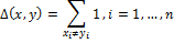
This method of comparing hash values is used in the DCT Based Hash method. The hash is 8 bytes in size, so the Hamming distance lies in the range [0, 64]. The smaller the value of Δ, the more similar the images.
To make comparison easier, the Hamming distance can be normalized using the length of the vectors:
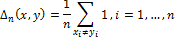
The normalized Hamming distance is used in the Simple Hash and Marr-Hildreth Operator Based Hash algorithms. The Hamming distance lies in the range [0,1], and the closer Δ is to 0, the more similar the images.
Let's define the correlation between two signals as:
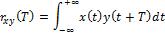
where x(t) and y(t) — are two continuous functions of real numbers. The function rxy(t) describes the offset of these two signals with respect to time T. The variable T determines how far the signal is shifted to the left. If the signals x(t) and y(t) are different, the function rxy T is called the cross-correlation function.
Let's define the Normalized Cross-Correlation Function:
Let xi and yi, where i = 0, … N − 1 – be two sequences of real numbers, and N – the length of both sequences.
We define the NCCF with delay d as:

where mx and my denote the mean value of the corresponding sequence.
The peak of the cross-correlation function (PCC) – is the maximum value of the function rd that can be achieved over the interval d = 0, N.
PCC is used to compare hash values in the Radial Variance Based Hash algorithm. PCC ∈ [0,1]; the larger its value, the more similar the images.
Types of edit distances
There are several basic edit distances. The main difference between them — is the set of operations that is allowed to be used.
The table below lists the most commonly used edit distances and the operations allowed for each of them.
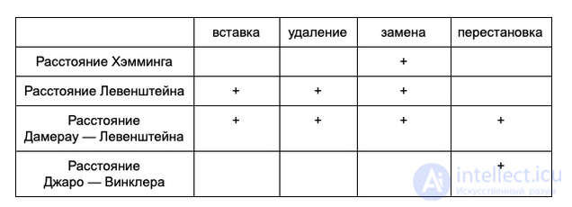
The Hamming distance allows only substitutions, so it can only be used to compare strings of the same length: we cannot lengthen a string via insertion or shorten it via deletion.
The Damerau—Levenshtein distance allows all four operations: substitution, insertion, deletion, and transposition of adjacent characters. Frederick Damerau showed that these four operations cover roughly 80% of writing errors.

Comments