
Lecture
Finite state machines as data structures
A finite state machine (FSM) is a set of states and a set of transitions that move from one state to another. One state is marked as the start state, and zero or more states are marked as final. A finite state machine is always in exactly one state.
Finite state machines are quite general and can be used to model a number of processes. For example, consider a slice of the daily life of my cat Koshi:
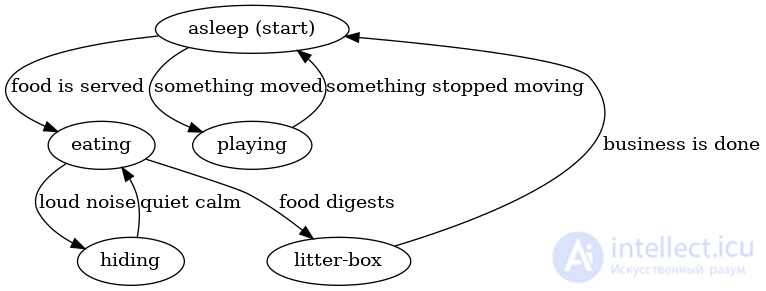
Some of the states are "sleeping" or "eating," and some of the transitions are "food is served" or "something moved." There are no final states here, because that would be needlessly grim!
Note that a finite state machine approximates our notion of reality. Koshi cannot play and sleep at the same time, so this satisfies our condition that the machine is always in only one state at a time. Also note that moving from one state to another requires only a single input from the environment. Namely, "falling asleep" does not remember whether it was triggered by being tired from play or by feeling satisfied after eating. No matter how Koshi fell asleep, he always wakes up if he hears something move or if the dinner bell rings.
Koshi's finite state machine can perform a computation given a sequence of inputs. For example, consider the following inputs:
If we apply these inputs to the machine described above, Koshi will pass through the following states in order: "sleeping," "eating," "hiding," "eating," "litter box." Consequently, if we observe that food was served, then a loud noise followed, then quiet calm followed, and finally Koshi's digestion, we could conclude that Koshi is currently in the litter box.
This particularly silly example demonstrates just how ordinary finite state machines really are. For our purposes, we will need to impose a few restrictions on the kind of finite state machine we use to implement our ordered set and map data structures.
An ordered set is like an ordinary set, except that the keys in the set are ordered. That is, an ordered set provides ordered iteration over its keys. Typically an ordered set is implemented with a binary search tree or a btree, while an unordered set is implemented with a hash table. In our case, we will look at an implementation that uses a deterministic acyclic finite state acceptor (FSA for short).
A deterministic acyclic finite state acceptor is a finite state machine that is:
How can we use these properties to represent a set? The trick is to store the keys of the set in the transitions of the machine. That way, given a sequence of inputs (that is, characters), we can determine whether a key is in the set based on whether the evaluation of the FSA ends in a final state.
Consider a set with a single key, jul. The FSA looks like this:

Consider what happens if we ask the FSA whether it contains the key "jul". We need to process the characters in order:
Since all the members of the key have been fed to the FSA, we can now ask: is the FSA in a final state? It is (note the double circle around state 3), so we can say that jul is in the set.
Consider what happens when we test a key that is not in the set. For example, jun:
The FSA cannot move because the only way out of state 2 is l, and the current input is n. Since l != n, the FSA cannot follow that transition. As soon as the FSA cannot move on some input, it can conclude that the key is not in the set. No further processing of the input is required.
Consider one more key, ju:
In this case the entire input is exhausted, and the FSA is in state 2. To determine whether ju is in the set, it must ask whether 2 is a final state or not. Since it is not, it can report that the key ju is not in the set.
It is worth pointing out here that the number of steps needed to confirm whether a key is in the set or not is bounded by the number of characters in the key! That is, the time required to look up a key has nothing to do with the size of the set.
Let us add another key to the set to see what it looks like. The following FSA represents an ordered set with the keys "jul" and "mar":
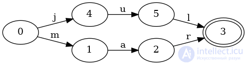
The FSA has become a little more complicated. The start state 0 now has two transitions: j and m. Consequently, given the key mar, it will first follow the m transition.
There is one more important thing to notice here: state 3 is shared between the jul and mar keys. Namely, two transitions enter state 3: l and r. This sharing of states between keys is really important, because it allows us to store more information in less space.
Let us see what happens when we add jun to our set, which has a common prefix with jul:
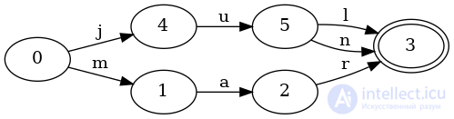
Do you see the difference? It is a small change. This FSA is very similar to the previous one. There is only one difference: a new transition, n, from state 5 to 3, has been added. Notably, the FSA has no new states! Since both jun and jul share the common prefix ju, those states can be reused for both keys.
Let us shake things up a bit and look at a set with the following keys: october, november, and december:

Since all three keys share the common suffix ber, it is encoded in the FSA only once. Two of the keys share an even longer suffix, ember, which is also encoded in the FSA exactly once.
Before moving on to ordered maps, we should take a moment to make sure that this really is an ordered set. Namely, given an FSA, how can we iterate over the keys in the set?
To demonstrate this, let us use the set we built earlier with the keys jul, jun, and mar:
We can enumerate all the keys in the set by traversing the entire FSA, following the transitions in lexicographic order. For example:
This algorithm is easy to implement with a stack of states to visit and a stack of the transitions that have been taken. It has O(n) time complexity in the number of keys in the set, with O(k) space complexity, where k is the size of the largest key in the set.
As with ordered sets, an ordered map is similar to a map, but with an ordering determined by the map's keys. Like sets, ordered maps are usually implemented with a binary search tree or a btree, while unordered maps are usually implemented with a hash table. In our case, we will look at an implementation that uses a deterministic acyclic finite state transducer (FST for short).
A deterministic acyclic finite state transducer is a finite state machine that (the first two criteria are the same as in the previous section):
In other words, an FST is like an FSA, but instead of answering "yes" / "no" for a given key, it answers either "no" or "yes, and here is the value associated with that key".
The set in the previous section needed only to store keys in the machine's transitions. The machine "accepts" an input sequence if and only if it is a key in the set. In this case, the map must do more than just "accept" an input sequence; it also needs to return the value associated with that key.
One way to associate a value with a key is to attach some data to each transition. Just as the input sequence is used to move the machine from state to state, an output sequence can be produced as the machine moves from state to state. This extra "power" makes the machine a transducer.
Let's look at an example of a map with a single element, jul, which is associated with the value 7:

This automaton is the same as the corresponding set, except that the first transition, j from state 0 to 1, has an output of 7 associated with it. The other transitions, u and l, also have outputs of 0 associated with them, which are not shown in the image.
As with sets, we can ask the map whether it contains the key "jul". But we also need to return the output. Here is how the machine processes a lookup of the key "jul":
Since all of the input has been fed to the FST, we can now ask: is the FST in a final state? It is, so we know that jul is in the map. In addition, we can report value as the value associated with the key jul, which is 7.
Not all that surprising, is it? The example is overly simplified. A map with a single key is not very instructive. Let's see what happens when we add mar to the map, associated with the value 3:
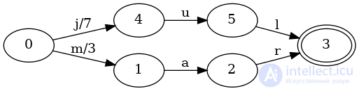
A new transition, m, with an output of 3, has grown out of the start state. If we look up the key jul, the process is the same as in the previous map: we return the value 7. If we look up the key mar, the process looks like this:
The only change here - apart from the different input transitions - is that 3 was added to value on the first move. Since all subsequent moves add 0 to value, the machine reports 3 as the value associated with mar.
Let's continue. What happens when we have keys with a common prefix? Consider the same map as above, but with the key jun added, associated with the value 6:
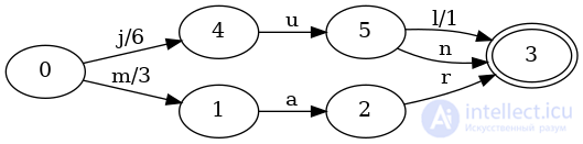
As with sets, an extra n transition was added, connecting states 5 and 3. But there were two more changes as well!
These changes to the outputs are really important, because now some details of looking up the value associated with the key jul change:
The final value remains 7, but we arrived at it differently. Instead of adding 7 on the initial j transition, we added only 6, but we made up the difference by adding 1 on the last l transition.
We should also convince ourselves that looking up the key jun is correct too:
The first transition adds 6 to value, but we never add anything more than 0 to value on the subsequent transitions. This is because the key jun does not go through the same final l transition as jul. Thus the two keys have different values, but we have done it in such a way that most of the data structure is shared between keys with common prefixes.
Indeed, the key property that makes this sharing possible is that every key in the map corresponds to a unique path through the machine. Consequently, there will always be some combination of transitions taken for each key that is unique to that particular key. All we have to do is figure out how to arrange the outputs along the transitions. (We will see how to do this in the next section.)
This sharing of outputs also works for keys with common prefixes and suffixes. Consider the keys tuesday and thursday, associated with the values 3 and 5, respectively (for the day of the week).

Both keys have the common prefix t and the common suffix sday. Note that the values associated with the keys also have a common prefix with respect to addition. Namely, 3 can be written as 3 + 0 and 5 can be written as 3 + 2. This idea is captured in the machine; the common prefix t has an output of 3, while the h transition (which is not in tuesday) has an output of 2 associated with it. Namely, when looking up the key tuesday, the first output t will be emitted, but the h transition will not be taken, so the output 2 associated with it will not be emitted. The remaining transitions have an output of 0, which does not change the final value emitted.
The way I have described the outputs may seem a bit restrictive; what if they are not integers? Indeed, the types of outputs that can be used in an FST are limited to things for which the following operations are defined:
Outputs must also have an additive identity I, such that the following laws hold:
Integers trivially satisfy this algebra (where prefix is defined as min), with the added benefit that they are very small. It is possible to create other types that satisfy this algebra, but for now we will work only with integers.
We needed to use only addition in the examples above, but we will need the two other operations to construct an FST. That is what we will cover next.
In the previous two sections, I tried to avoid talking about building the finite state machines used to represent ordered sets or maps. Namely, construction is a bit more complicated than simple traversal.
To keep things from getting too complicated, we impose a restriction on the elements in our set or map: they must be added in lexicographic order. This is a burdensome restriction, but later we will see how to relax it.
To motivate the construction of finite state machines, let's talk about tries.
Trie construction
A trie can be viewed as a deterministic acyclic finite state acceptor. Therefore, everything you learned in the previous section about ordered sets applies to them as well. The only difference between a trie and the FSA shown in this article is that a trie allows sharing of prefixes between keys, whereas an FSA allows sharing of both prefixes and suffixes.
Consider a set with the keys mon, tues and thurs. Here is the corresponding FSA, which benefits from sharing both prefixes and suffixes:
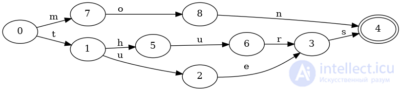
And here is the corresponding trie, which shares only prefixes:
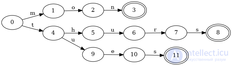
Note that there are now three distinct final states, and the keys tues and thurs require duplicating the last s transition to the final state.
Building a trie is fairly simple. Given a new key to insert, all you have to do is perform an ordinary lookup. If the input is exhausted, then the current state should be marked as final. If the machine stops before the input is exhausted because there are no valid transitions to follow, simply create a new transition and node for each remaining input symbol. The last node created should be marked as final.
FSA construction
Recall that the only difference between a trie and an FSA is that an FSA allows sharing of suffixes between keys. Since a trie is itself an FSA, we could build a trie and then apply a general minimization algorithm, which would achieve our goal of sharing suffixes.
However, general minimization algorithms can be expensive in both time and space. For example, a trie can often be much larger than an FSA that shares structure between the suffixes of keys. Instead, if we can assume that keys are added in lexicographic order, we can do better. The essential trick is to realize that when a new key is inserted, any parts of the FSA that do not share a prefix with the new key can be frozen. Namely, no new key added to the FSA can reduce that part of the FSA.
Some images may help explain this better. Consider the keys mon, tues and thurs again. Since we must add them in lexicographic order, we will add mon first, then thurs, and then tues. Here is what the FSA looks like after adding the first key:

This is not all that interesting. Here is what happens when we insert thurs:

Inserting thurs caused the first key, mon, to be frozen (shown in blue in the image). Once a particular part of the FSA has been frozen, we know that it will never need to be changed in the future. Namely, since all future keys will be added >= thurs, we know that no future keys will begin with mon. This is important because it allows us to reuse this part of the automaton without worrying about whether it might change in the future. In other words, the states colored blue are candidates for reuse by other keys.
The dashed lines represent the fact that thurs has not yet been added to the FSA. Indeed, adding it requires checking whether there are any reusable states. Unfortunately, we cannot do that yet. For example, it is true that states 3 and 8 are equivalent: both are final and neither has any transitions. However, it is not true that state 8 will always be equal to state 3. Namely, the next key that we might add could, for example, be thursday. This would change state 8 to have a d transition, making it not equal to state 3. Thus, we cannot yet reach a final conclusion about what the key thurs looks like in the automaton.
Let's move on to inserting the next key, tues:
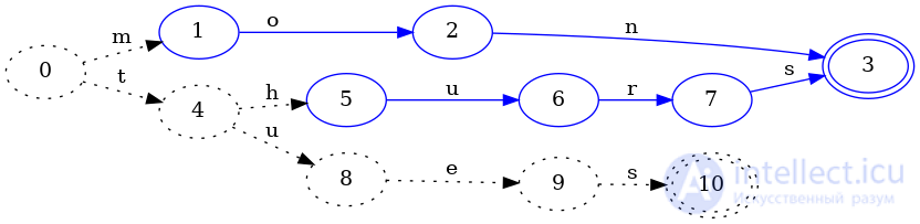
In the process of adding tues, we concluded that the hurs part of the key thurs could be frozen. Why? Because no future key can minimize the path traveled by hurs, since keys are inserted in lexicographic order. For example, we now know that the key thursday can never be part of the set, so we can conclude that the final state of thurs is equivalent to the final state of mon: they are both final and both have no transitions, and this will always be true.
Note that state 4 remains dashed: it is possible that state 4 could change with subsequent key insertions, so we cannot yet consider it equal to any other state.
Let's add one more key to drive the point home. Consider inserting zon:
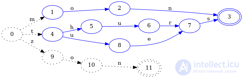
Here we see that state 4 has finally been frozen, because no subsequent insertion after zon can change state 4. In addition, we can also conclude that thurs and tues share a common suffix, and that, indeed, states 7 and 9 (from the previous image) are equivalent, because neither is final and both have a single transition with input s that points to the same state. It is very important that both of their s transitions point to the same state, otherwise we could not reuse the same structure.
Finally, we must report that we are done inserting keys. Now we can freeze the last part of the FSA, zon, and look for duplicate structure:
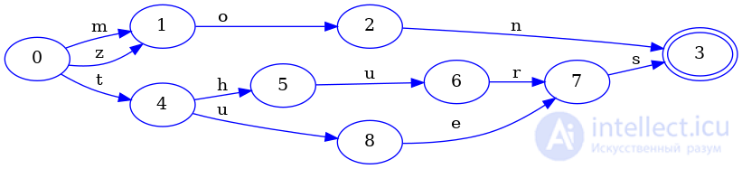
And sure enough, since mon and zon share a common suffix, there really is redundant structure. Namely, state 9 in the previous image is in all respects equivalent to state 1. This is true only because states 10 and 11 are also equivalent to states 2 and 3. If that were not the case, then we could not consider states 9 and 1 equal. For example, if we had inserted the key mom into our set and still assumed that states 9 and 1 were equal, the resulting FSA would look something like this:

And that would be wrong! Why? Because this FSA would claim that the key zom is in the set, but we never added it.
Finally, it is worth noting that the construction algorithm described here can run in O(n) time, where n is the number of keys. It is easy to see that the initial insertion of a key into the FST, without checking for redundant structure, takes no longer than a loop over each character in the key, assuming that finding a transition in each state takes constant time. A harder question is how to find redundant structure in constant time. The short answer is a hash table, but I will explain some problems with it in the section on construction in practice.
FST construction
Construction of deterministic acyclic finite state transducers works in much the same way as construction of deterministic acyclic finite state acceptors. The key difference is the placement and sharing of outputs on transitions.
To keep the mental burden low, we will reuse the example from the previous section with the keys mon, tues and thurs. Since we are building a map, we will associate the numeric day of the week with each key: 2, 3 and 5, respectively.
As before, let's start by inserting the first key, mon:

(Recall that dashed lines correspond to parts of the FST that may change on a subsequent key insertion.)
This is not very interesting, but it is at least worth noting that the output 2 is placed on the first transition. Technically, such a transducer would be no less correct:

However, placing outputs as close to the start state as possible makes it much easier to write an algorithm that shares output transitions between keys.
Let's move on to inserting the key thurs, mapped to the value 5:

As in the FSA construction, inserting the key thurs lets us conclude that the mon part of the FST will never change. (Shown in blue in the image.)
Since the keys mon and thurs have no common prefix, and they are the only two keys in the map, all of their output values can be placed on the first transition out of the start state.
However, when we add the next key, tues, things get a bit more interesting:
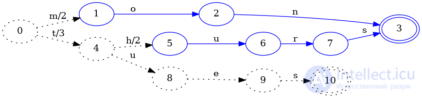
As in the FSA construction, this identifies another part of the FST that can never change, and freezes it. The difference here is that the output on the transition from state 0 to 4 changed from 5 to 3. This is because the value of the key tues is 3, so if the initial t transition added 5 to the value, the value would be too large. We want to reuse as much structure as possible, so when we determine a common prefix, we also look for a common prefix in the output values. In this case, the prefix of 5 and 3 is 3. Since 3 is the value associated with the key tues, all of its remaining transitions can have an output of 0.
However, if we change the output of the 0->4 transition from 5 to 3, the value associated with the key thurs will now be wrong. We must then "push" the remainder of the value, after the prefix of 5 and 3, further down. In this case, 5 - 3 = 2, so we add 2 to each transition out of 4 (except for the new u transition that we added).
In this way, we preserve the outputs of the previous keys, add a new output for the new key, and share as much structure as possible in the FST.
As before, let's try adding one more key. This time let's pick a key that affects the outputs in a more interesting way. Let's add tye to the map and associate it with the value 99 to see what happens.
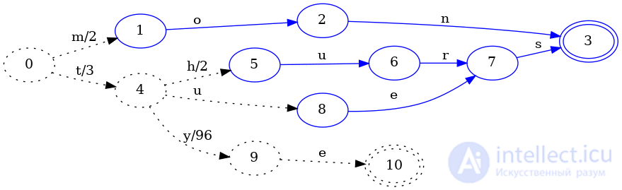
Inserting the key tye allowed us to freeze the es part of the key tues. In particular, as in the FSA construction, we identified equivalent states so that thurs and tues could share states in the FST.
The difference in the FST construction is that the output associated with the 4->9 transition (which was just added for the key tye) has an output of 96. It chose 96 because the transition before it, 0->4, has an output of 3. Since the common prefix of 99 and 3 is 3, the output of 0->4 is left unchanged, and the output for 4->9 is set to 99 - 3 = 96.
For completeness, here is the final FST after indicating that no more keys will follow:
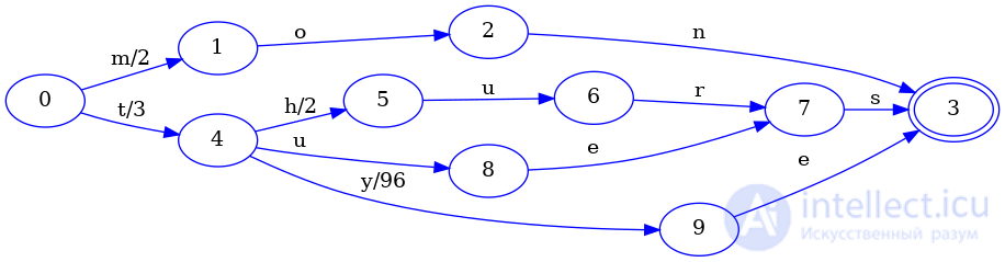
The only real difference from the previous step is that the last transition of the key tye is connected to the final state shared by all the other keys.
Construction in practice
Actually writing code to implement the algorithms described above is beyond the scope of this article. (A fast implementation of it is, of course, freely available in my fst library.) However, there are some important issues worth discussing.
One of the most important use cases of the FST data structure is its ability to store and search a very large number of keys. This goal somewhat conflicts with the algorithm described above, since it requires that all frozen states be kept in memory. Namely, to determine whether there are parts of the FST that can be reused for a given key, you must be able to actually look up equivalent states.
The literature describing this algorithm (referenced in the next section) says that a hash table can be used for this, which provides constant-time access to any particular state (assuming a good hash function). The problem with this approach is that a hash table typically incurs some overhead on top of actually storing all of the states in memory.
The heavy memory cost can be reduced by sacrificing the guaranteed minimality of the resulting FST. Namely, one can maintain a hash table of bounded size. This means that frequently reused states are kept in the hash table, while less frequently reused states are evicted. In practice, a hash table with about 10,000 slots provides a decent trade-off and comes close to minimality in my own unscientific experiments. (The actual implementation is a bit better and stores a small LRU cache in each slot, so that if two common but different nodes map to the same bucket, they can still be reused.)
An interesting consequence of using a bounded hash table that stores only some of the states is that FST construction can be streamed to a file on disk. Namely, when states are frozen, as described in the previous two sections, there is no reason to keep all of them in memory. Instead, we can write them out immediately to disk (or a socket, or whatever).
The end result is that we can build an approximately minimal FST from presorted keys in linear time and constant memory.
References
The algorithms presented above are not my own. (As far as I know, I came up with the idea of LRU caching. But that is all!)
I got the FSA construction algorithm from Incremental Construction of Minimal Acyclic Finite State Automata. In particular, section 3 explains the details well enough, but overall the paper is a good read.
I got the FST construction algorithm from Direct Construction of Minimal Acyclic Subsequential Transducers. The whole paper is a really good read, but I had to reread it 3-5 times over the course of a week for it to really sink in. At the end of the paper there is pseudocode for the algorithm, which is easy to read once your brain gets used to what all the variables mean.
These two papers pretty much cover everything that was in the article. However, to write an efficient implementation, it is worth reading more. In particular, this article does not go into detail about how nodes and transitions are represented in an FST. The short answer is that the FST representation is a sequence of bytes in memory, and the vast majority of states take up exactly one byte of space. Indeed, the representation of finite state machines is an active area of research. Here are the two papers that helped me the most:
For an excellent but very detailed and in-depth overview of the field, Jan Daciuk's dissertation is great (beware: it is a compressed PostScript file).
For a short and pleasant experimentally motivated overview of construction algorithms, Comparison of Construction Algorithms for Minimal, Acyclic, Deterministic, Finite-State Automata from Sets of Strings works very well.

Comments