Simple Automata: Deterministic and Probabilistic Automata

1 Basic concepts and definitions

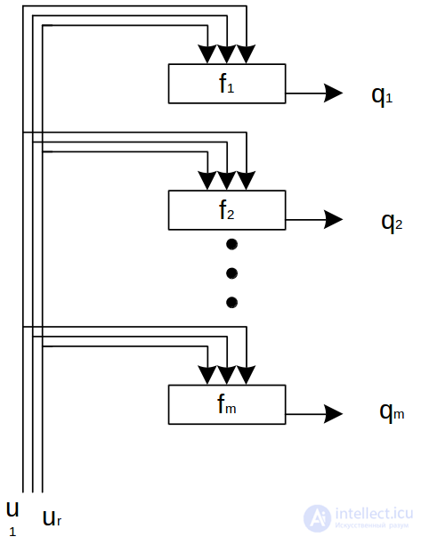
Suppose there are several logical variables u₁…u_r, and let us treat them as a vector U. Let f be a logical function of these variables that forms some complex logical statement

q=f(U)

We will treat q as the output value of a relay-contact circuit (RCC) that implements the logical function f.

RCCs encountered in practice, as a rule, have not one output but several, and each output implements its own logical function.

We will assume that an RCC performs logical operations instantaneously, i.e. if at time t the vector U arrives at the input of the circuit, then the corresponding value q=f(u) is obtained at the output at the very same moment. To describe the operation of an RCC over time, it is convenient to introduce the concept of discrete time. That is, we replace the physical notion of infinite, uniform, and continuously flowing time with point-like moments of time, assuming that all changes occur precisely at these moments and that nothing changes between them. Moreover, we assume that the length of these intervals is so small that it can be neglected. On the t axis we mark the moments at which the input value may change: t₁, t₂, …, t_n. These values are called clock cycles. The equation q[n]=f(u[n]), where n is the n-th clock cycle, describes the operation of an RCC over time. An RCC is the simplest kind of finite automaton – a finite automaton without memory.

Finite automata are usually specified not by equations but by transition and output tables or by the transition graph of the finite automaton. In the transition table, the rows correspond to different input signals and the columns to different states of the automaton. At the intersection of a row and a column is the state to which the automaton passes.

Another way of specifying a finite automaton, which provides greater clarity, is to specify the automaton by means of a directed graph. The vertices of the graph are the possible states of the automaton. Vertices i and k are connected by arcs if and only if there exists a signal that takes the automaton from state i to state k; the arc is labeled with the value of the signal U, and the value of the output signal q is given in parentheses.

We will call the signal U the influence of the environment. The environment is described by the probability of one event or another occurring. That is, the environment E is described by the set of its states D and the probability P of exactly that state occurring. Let us assume this.

2 The concept of a stationary and a dynamic environment.

Before we begin to construct and describe any automata, let us define such a fundamental concept of the theory of simplest automata as the concept of the environment. Unlike in the natural sciences, in the theory of simplest automata the environment interests us from only one point of view: its reaction to the actions of our automaton. The values of the evaluations of the automaton's actions are described by some finite set D= {d₁,d₂, …d_n}. If our automaton can perform at the i-th clock cycle one of m actions, then the environment is described by a probability matrix A(m,n), in which A(i,j) = the probability of the j-th reaction of the environment (d_j) to the i-th action of the automaton. If over time the values of the matrix A remain unchanged, the environment is called stationary.

This interesting interpretation of the behavior of biological organisms and description of the conditions of their existence was proposed by the brilliant Soviet mathematician and engineer M.L. Tsetlin. The essence of Tsetlin's simplicity hypothesis is that any sufficiently complex behavior is composed of a set of simple behavioral acts. Their joint realization and simplest interaction with the environment result in very complex behavioral processes.

Let us consider one of the simplest biological experiments, on the basis of the results of which Tsetlin created his first automata. In biology these experiments are known as Yerkes' experiments. At the beginning of the experiment an earthworm was placed on a brightly lit platform of a "T-shaped" maze. The worm began to move in order to find more comfortable conditions of existence. Where the corridor branched, the worm had a choice of two alternatives. Of course, the worm could not know that an electric field was switched on along the left corridor, and that the corridor ended in a salt bath that irritated the worm. Meanwhile, the right corridor led the worm to a darkened, damp chamber where it felt excellent.

In the course of the experiment the worm repeatedly traveled this path and "made a decision" about which corridor to choose, gradually learning to choose only the right corridor. In other words, having no initial information about the features of its habitat, the worm, in the process of interacting with the surrounding world, worked out a purposeful way of behaving in it.

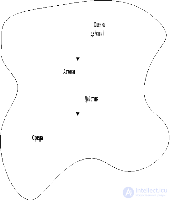
From Tsetlin's point of view, the general scheme of this experiment looks as follows.

How, then, are this automaton and its habitat described? Our automaton has two possible actions: {"Right", "Left"}, and the environment also has two reactions: {"Punishment", "Reward"}. The probability matrix will look like this:

Let us change the conditions of the experiment slightly. These experiments were described by Thorndike. As in the first experiment, a rat is placed in a T-shaped maze. Food is placed at the end of both the right and the left corridor. But on the way to the food, in both corridors, the rat encounters unpleasant sensations from electric shock. These shocks occur with fixed probabilities P_r and P_l, which do not change during a single series of experiments. The goal of the experiment is to determine whether the rat, in the course of learning, can learn to choose the corridor leading to the food in which the probability of electric shock is lower. With a noticeable difference between P_r and P_l, after a more or less lengthy period of learning, the rats assessed this difference correctly and made a sensible decision about which route to choose. The probability matrix for this experiment will look like this:

From the point of view of the theory of simplest automata, both cases are examples of a stationary environment. But such a world is possible only in an experiment. The processes occurring in nature are considerably more complex and diverse. How can they be described?

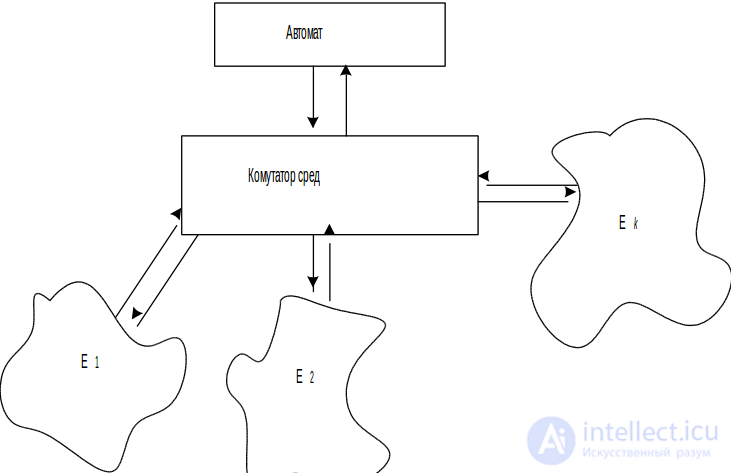
The description of more complex habitats and of the "life" of automata is associated with the concept of a dynamic environment. Since the laws governing changes in the parameters of the external environment can be very different, we will consider the simplest way of describing a dynamic environment. We will treat a dynamic environment as a set of a finite number of stationary environments, described in the way already familiar to us, E₁, E₂ … E_k. And we will assume that each of these environments is an instantaneous snapshot of the state of the dynamic environment. These snapshots, changing like frames of a film, recreate the dynamic environment for us. The scheme of interaction of the automaton with such an environment looks like this:

The switch, as it were, connects the automaton to one stationary environment or another. Both the characteristics of these environments and the laws of operation of the switch are not known to the automaton in advance. Adaptation consists not only in estimating the probabilities P_i^m, where the superscript denotes the environment E_m, but also in determining the pattern by which the environments change.

+We will consider only one, the best-studied, special case of the operation of the switch. We will assume that the switch changes environments guided by some square matrix. Let us call it the probabilistic environment-switching matrix T. T_ij is the probability of transition from E_i to E_j at the next step. By the laws of probability theory

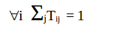
Such a dynamic environment is also called switching.

The concept of purposeful behavior of an automaton.

When evaluating the behavior of automata, whose design we will discuss later, we will often speak of purposefulness of behavior. First, let us discuss this concept from the standpoint of everyday logic.

A fox has come back with rich prey. Part of it has fed the fox's brood, and the fox hides the remaining food "for a rainy day". She carefully digs a hole, puts the meat into it and covers it with earth. Watching the fox's behavior, one might conclude that the goal of her actions is generated by her "intellect". Her behavior is so purposeful and "reasonable".

But the fate of our heroine turned out to be not very happy. She fell into a trap and became a resident of a zoo. Now she no longer has to spend effort on obtaining food. The keepers feed her. But what is a fox to do when there is a surplus of food? Hide it, of course! And the fox scratches the concrete floor of the enclosure with her claws, and after a while, when the "hole" is ready, she "hides" the meat in it. After that she stops noticing the rest of the meal, which, of course, remains lying on the floor of the enclosure. The fox simply ignores it and does not see the "buried" meat. What looked purposeful in the animal's familiar environment becomes devoid of any features of reasonableness under the conditions of a different reality.

Such narrowly specialized actions, closely tied to a typical situation in the surrounding world, are usually called reflexes. The simpler the organism is organized, the more rigid the reflex scheme is. The more absurd its behavior looks in a changed environment.

How, then, should one evaluate the purposefulness of behavior of artificially constructed automata? To do this, let us replace our automaton with a device that chooses actions with equal probability. At each step of its operation, this mechanism, taking no account of the "penalty" - "reward" signals arriving at its input, chooses one of the actions available to it with the same probability, equal to 1/n.

W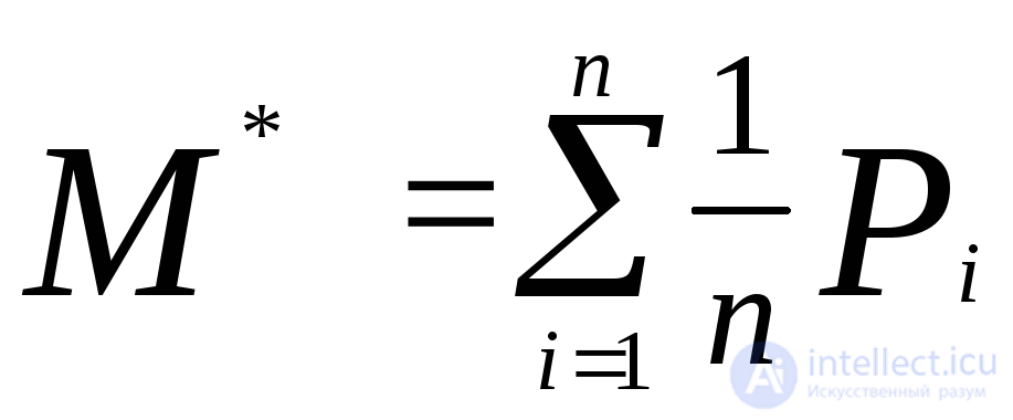ith infinite repetition of the experiment with the equiprobable action-selection mechanism, a certain total penalty will be accumulated. Its value is determined as the mathematical expectation of the penalty by a formula well known from probability theory:

The value of M^* makes it possible to interpret the concept of purposeful behavior as follows. We will say that an automaton behaves purposefully if the total penalty it has accumulated is smaller than in the case of using the equiprobable action-selection mechanism. And we will consider behavior non-purposeful if this total penalty is greater than or equal to M^*.

Suppose, for example, that in Thorndike's experiment P_r= 0.9, and P_l= 0.4. If the rat knew these probabilities in advance, it would of course always prefer to run into the left corridor. If, with our values of the penalty probabilities for the actions, the rat is placed under conditions of equiprobable choice, then its total penalty will be equal to

M = 0.5*0.9 + 0.5*0.4 = 0.65

And the best behavior is the one at which the total penalty reaches its minimum (when only the left corridor is chosen). In this case

M = 0*0.9 + 1*0.4 = 0.4

+Let us describe the structure of technical devices that ensure purposeful behavior in any stationary environment that is not known a priori.

4 The deterministic automaton

Example: Consider a situation found in folk tales. Ivanushka the Fool meets a wedding. And he starts loudly lamenting and crying. Such inappropriate behavior causes an instant reaction from the environment. Cruelly beaten, Ivanushka after some time meets a funeral. Remembering his failure, he starts laughing merrily and singing. And again a cruel punishment befalls our simple-hearted hero. He is beaten again.

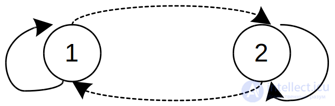
Let us draw the transition graph of this automaton. State 1 is dancing, state 2 is crying. Our environment can also give only two responses: "Beat" or "Do not beat". The solid line denotes the reaction of our automaton to a reward (the "Do not beat" response); the dashed line denotes its reaction to a punishment (the "Beat" response).

Let us build a transition table for this example.

The rows are the state of the automaton at time t

U is the state of the environment. Both of these variables are binary.

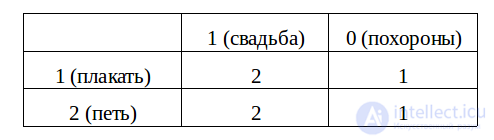
Values of the variable X: "1" – crying, "2" - singing

Values of the variable U: "0" – funeral, "1" - wedding

We will take the output of this automaton to be the information about a change of the automaton's state. "0" – if it does not change state

"1" – if it changes.

Analyzing Ivanushka's hard fate, the idea immediately arises that his behavior would be more appropriate if, when making a decision, Ivanushka relied on the data of several of the most recent events, i.e. if he had memory.

This is what the transition graph of such an automaton looks like. A solid arrow shows the transition on punishment, a dashed one on reward. In our example three stable states are defined for each action of the automaton. We will assume that states 1, 2, 3 denote the action "crying" of our Ivanushka, and states 4, 5, 6 the action "singing". This number is called the memory depth of the finite automaton or the degree of its inertia. Let us show that such an automaton will fairly quickly find the best action for a static environment and will perform only that action. Let us clarify this idea. Suppose that at the beginning our automaton is in state 3. And the influence of the environment is described by (0.9; 0.1), i.e. with probability 0.9 he meets a wedding and with probability 0.1 a funeral. Let us observe the behavior of our Ivanushka. With probability 0.9 he meets a wedding, and Ivan is beaten, he moves to state 4, he starts singing and again with probability 0.9 meets a wedding. By probability theory, the probability of getting two weddings in a row from the environment is 0.81, two funerals in a row 0.01, and the probability of one wedding and one funeral = 0.18. Consequently, after two interaction steps the automaton will be in state 1 with probability 0.01, in its previous position with P=0.18, and in state 5 with P=0.81. As the number of interactions grows, the picture does not change qualitatively. The probability of leaving the group 6-4 steadily falls, while the probability of staying in it grows.

What will happen next? With P=0.9 our automaton will receive a reward and move to state 6, and so on. The probability of leaving the group 4-6 will keep decreasing. This process is very similar to a learning process, after which our automaton behaves "fairly adequately" in the given static environment. "Fairly adequately" because there is a very small but nonzero probability of leaving the group of the most favorable behavior (i.e. behavior in which the sum of penalties is minimal).

If the environment is dynamic, then there is a dependence between the probability of a change in the laws of the environment and the memory depth of the automaton. This statement is intuitively clear, since in a dynamic world situations change very frequently, and inertia can hardly serve as a good means of existing in this world. It has been shown experimentally that each dynamic world requires its own best memory depth, chosen depending on the rate of change of the situation, and not by the principle "the more, the better". Such a memory depth is called optimal.

All of the above is also true for an automaton with more than two actions and more than two states of the environment. The greater the memory depth of such an automaton, the more purposeful its behavior. The automaton we have considered is called an automaton with linear tactics.

Let us stress once more that increasing the memory depth improves the purposefulness indicator of an automaton with linear tactics for static environments. Moreover, Tsetlin showed that if minP_i<0.5, then as the memory depth qof the automaton with linear tactics increases, we obtain a sequence of automata with linear tactics with ever increasing memory depth that is asymptotically optimal. This means that as q→∞, M(q, E) → M_min– the minimal total penalty. Thus the construction proposed by Tsetlin ensures, for sufficiently large values of q, behavior arbitrarily close to the best in any stationary random environments.

Let us consider a couple more designs of automata with linear tactics.

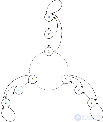
This design was proposed by V.I. Krinsky. We will call it "trusting". This is what its transition graph looks like.

When a penalty signal arrives, the behavior of this automaton is similar to that of Tsetlin's automaton with linear tactics, but when a reward signal is received, this automaton, regardless of which state of the petal it is currently in, moves to the deepest state of that petal. This automaton seems inclined to believe in the good, and a positive signal from the environment brings it into a state of "euphoria".

It has been rigorously proved that Krinsky's automata behave purposefully in any stationary random environments.

One may get the impression that any measures to increase the inertia of an automaton improve the purposefulness indicator of its behavior.

+The situation changes qualitatively if our linear automaton deals with a dynamic environment. If environments change sufficiently fast, inertia can hardly serve as a good means of existing in this world. After all, in a dynamic world one must quickly track the changes that arise in the environment, and every dynamic world requires its own memory depth, chosen depending on the rate of change of the situation.

5 The probabilistic automaton

Let us now describe the structure of an automaton whose behavior will, to one degree or another, meet the requirements of the environment. This automaton is called probabilistic. It is built similarly to an automaton with linear tactics, but its transition and output functions are random functions. That is, the probabilities of transitions from one state to another are specified when a certain signal arrives at the input. Such an automaton is, as a rule, specified by a system of matrices in which, at the intersection of the i-th column and the k-th row, the probability P of the transition from the i-th state to the k-th is given. In the special case when such matrices contain only "0" and "1", the already familiar deterministic automaton is described.

Writing out such matrices is too cumbersome a procedure, so let us show the form of these matrices for the automaton shown in the figure.

These matrices define the deterministic structure of our automaton. P+ is the transition matrix when a reward signal arrives, and P- when a penalty signal arrives.

The matrices of the example describe a probabilistic automaton, sometimes also called Krylov's automaton. When a reward signal arrives, this automaton acts like a deterministic automaton, and when a penalty signal arrives, it stays in its previous position with probability 0.5 and moves to another state with probability 0.5. Such an automaton seems in no hurry to change its action, and makes the decision to move randomly (but in a way that does not change as the automaton works), having first "tossed a coin". Such an automaton can also be called cautious.

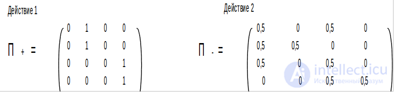
Let us give an illustrative example of such an automaton.

Consider an attempt to formalize the ways a night moth escapes from a bat. The bat emits a directional ultrasonic signal and is able to pick up the reflected signal, and with fairly high accuracy it can distinguish and identify signals, telling moving targets from stationary ones, ground targets from airborne ones, small from large. In addition, the reflected signal allows the bat to determine the direction and distance to potential targets with very great accuracy.

Night moths are also able to receive the bat's signal and determine its intensity. The moth's behavior differs depending on how far away the bat is. We will distinguish three maneuvers of the moth.

1. The moth started moving in the direction opposite to its previous movement.

2. The moth changed direction in the vertical plane, departing from its previous course upward or downward.

3. The moth started chaotic movement, i.e. switched to a flight trajectory that makes it as hard as possible for the attacker to predict the next point on this trajectory.

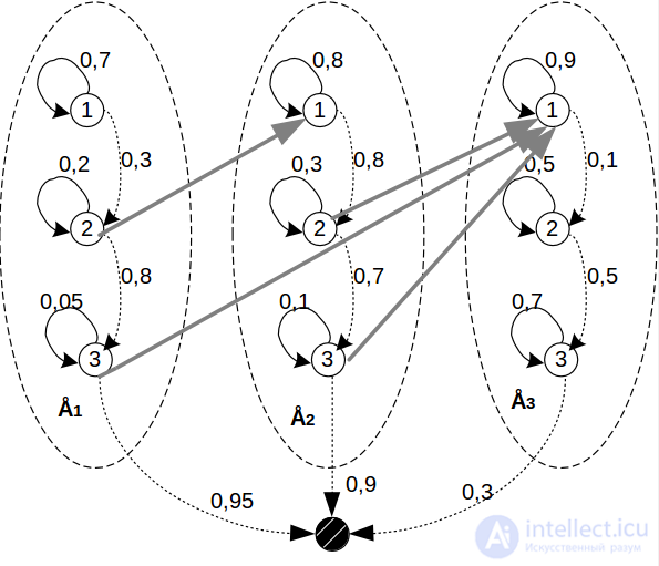
The figure shows the state transition graph of a probabilistic automaton. Its peculiarity is that for each group of states (they are circled with a dashed line in the figure) there is a nonzero probability of moving to a special state describing the death of the automaton. State 1 can be interpreted as follows: 1 – with P=0.3 the bat detects the moth, and with P=0.7 it misses it. 2 – the bat determines the direction of its movement and with P=0.8 the target is not lost. 3 – the bat catches up with the moth and destroys it with P=0.95. What can the moth oppose to the pursuer? For simplicity of exposition, we will consider each of the groups of states of the automaton as a certain environment, defined by the moth's strategy. E1 is straight flight. E2 is a change of direction of movement in the horizontal or vertical plane, and E3 is chaotic movement. The moth's actions amount to changing environments, switching between them. In this case the automaton can perform an action only in state 2 or 3. This is shown in the figure by double transition arrows.

Build the state table of this automaton yourself.

+In the given example, the actions that allow the moth to maximally increase its probability of survival are quite simple and transparent. In the general case, however, choosing the optimal sequence of switchings of the automaton's actions that maximizes its lifetime is far from trivial. Our goal, to show the principles of operation of the probabilistic automaton, has been achieved.

6 The automaton with variable structure

To begin with, consider the following situation. Suppose that you get from home to work every day in your car. You have two possible routes at your disposal, and you are free to choose either one. Since you always leave at the same time, the situation on each route is, as it were, stationary. And analyzing this situation, you have become convinced that one of the routes is better than the other: less time is spent, the traffic here is lighter than on the other route, and there are not so many traffic lights either. But here is the trouble: from time to time, because of some repair work, the speed of traffic here drops sharply, traffic jams form, and you can lose a lot of time until they clear. In these conditions this route becomes much worse than the other. You would lose much less time by choosing the other route on these unlucky days. If there is no information about how often repair work occurs on the first route, then when leaving home you have no chance of guessing which route is better to take today. However, day after day you accumulate information. You learn from your bitter experience. It turns out that traffic jams most often form on Wednesday and Friday, and the probability of these jams is quite high. Then, choosing the first route on the other days of the week, on Wednesday and Friday you unhesitatingly choose the less good route.

But neither the automaton with linear structure nor Krylov's probabilistic automaton can adapt to a frequently changing dynamic environment, since its transition tables do not change in the course of operation. Therefore let us consider a model of an automaton with variable structure. This is the already familiar probabilistic automaton which, at the start of operation, is in a neutral state, with transition probabilities set in advance.

If, after performing some action, the automaton has received a penalty signal, then in the transition matrix it decreases the value of the probability of this transition by a given amount Δ , but the sum of all elements of a row must equal 1, so all nonzero elements of the row must be changed by the amount Δ/h, where h is the number of nonzero elements of the row.

S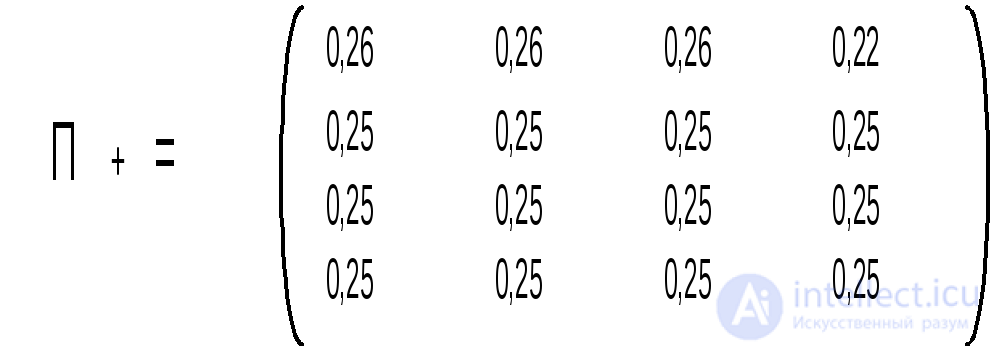uppose, for definiteness, that at the initial moment the automaton was in state 1 and performed action 1 corresponding to this state. By an equiprobable choice according to matrix P+ it moved to state 4. And suppose that after this it received a penalty signal. Receiving such a signal makes the automaton consider its transition 1 – 4 a mistake. This information is recorded as follows. The probability P⁺₁₄ decreases by Δ, and all the other elements of the row increase by Δ/3. For convenience let us take Δ= 0.03. Then after this step matrix P- will not change, and matrix P+ will look like this:

At the next step the automaton performs action 2, corresponding to state 4, and chooses the next state on the basis of matrix P- (since in the current act of interaction with the environment it is under the conditions of the last signal from the environment – a penalty).

S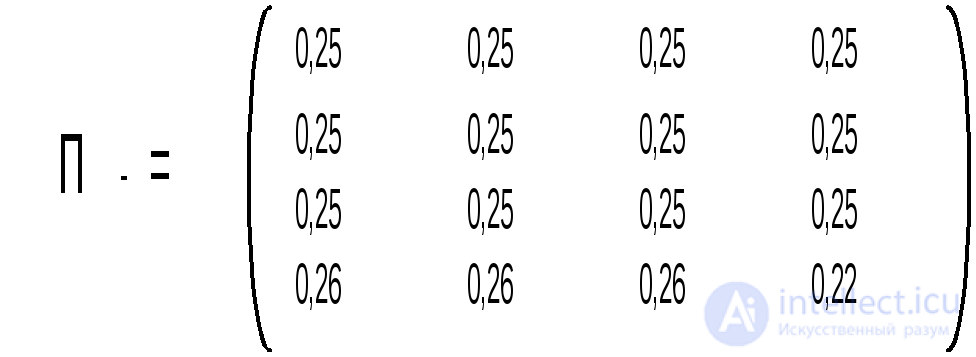uppose it chose the transition 4 – 4 and again received a penalty. Now matrix P- changes, while matrix P+ remains unchanged.

Thus, matrices P+ and P- are gradually rebuilt depending on the signals produced by the environment. For automata with variable structure the following fundamental result has been shown experimentally: over time, the operation of an automaton with variable structure in switching environments, in which an automaton with linear tactics behaves purposefully, approaches without bound the behavior of an automaton with linear structure and optimal memory depth. In other words, an automaton with variable structure finds the optimal memory depth by itself. This is very important, since the value of the optimal memory depth cannot be determined analytically; it is selected in the course of operation in the environment.

We will limit ourselves to considering this design of an automaton.

Let us only say that there is a very large set of classes of finite and infinite automata actively used in engineering. And you will discuss these objects in more detail in courses on automatic control theory. I would now like to summarize what has been said.

From a mathematical point of view, an automaton is specified by A – the input alphabet, B – the output alphabet, S – the alphabet of states of the automaton, and two functions: φ - the transition function and β - the output function.

Recall that an alphabet means a set of possible values. φ and β can also be arbitrary relations and probabilistic functions.

It should be clearly understood that the function φ maps the set SxA into S; and β maps the set SxA into B.

See also

• [[b7814]]
• [[b9799]]
• [[b7813]]
• [[b6894]]
• [[b7816]]
• [[b9261]]
• [[b7819]]
• Mealy machine
• Moore machine
• JFLAP — a cross-platform simulator program (for automata, Turing machines, grammars)
• Automata-based programming
• Sequential Function Chart
• Compiler
• Translator
• Petri nets
• Sequential logic
• Decision table
• Suffix automaton

See also

• 5.2. State Machine Representation
• Simple Automata: Deterministic and Probabilistic Automata
• five . State machines 5.1. Concept of automaton
• The concept of cellular automata. Types and sequences of cellular automata
• 5.4. Equivalence of finite automata: Moore's theorem
• Finite State Machines as Data Structures for Indexing Keys
• 5.7. Examples of finite automata