
Lecture
The FST command line tool
I created the FST command line tool as a way to easily play with data and as a demonstration of how to use the underlying library. I do not intend for it to be particularly useful in itself, but in this blog post it will serve as a way of running experiments on real data.
In this section, I will give a very brief overview of the command and then move straight on to experiments with real data.
If you do not want to play with the tool, you do not have to download it. Namely, in this section I generally show the commands I run, along with their results, wherever possible.
Currently, the only way to get the command is to compile it from source. To do that, you first need to install Rust and Cargo . (The current stable version of Rust will work. The release distribution includes both Rust and Cargo.)
Once Rust is installed, clone the fst repository and build it:
$ git clone git://github.com/BurntSushi/fst
$ cd fst
$ cargo build --release --manifest-path ./fst-bin/Cargo.toml
On my fairly powerful system, compilation takes just under a minute.
After compilation completes, the fst binary will be located at ./fst-bin/target/release/fst.
The fst command line tool has several commands. Some of them serve a purely diagnostic role (for example, "I want to look at a particular state in the underlying transducer"), while others are more utilitarian. In this article we will focus on the latter.
Here are the commands:
The set and map commands are crucial because they provide the means to create FSTs from simple data.
Let's start with a simple example that we can easily visualize. Consider a map from a month abbreviation to its numeric position in the Gregorian calendar. Our raw data is a simple CSV file:
jan,1
feb,2
mar,3
apr,4
may,5
jun,6
jul,7
aug,8
sep,9
oct,10
nov,11
dec,12
We can build an ordered map from this data with the fst map command:
$ fst map months months.fst
If our data were already sorted, we could pass the --sorted flag:
$ fst map --sorted months months.fst
The --sorted flag tells the fst command that it can build the FST in a streaming fashion, which is very fast. Without the --sorted flag, it must sort the data first.
If we want to visualize the underlying transducer, it is easy if you have graphviz installed (which provides the dot command used below):
$ fst dot months.fst | dot -Tpng > months.png
$ $IMAGE_VIEWER months.png
And you should see something like this:
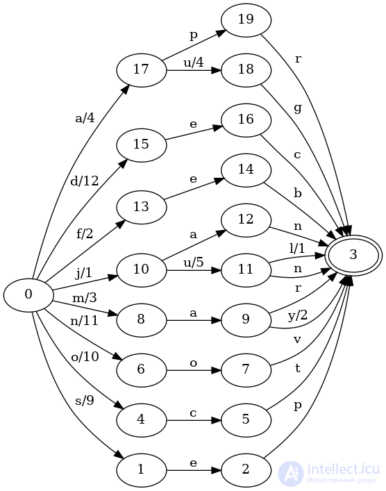
Since the data set is small, searching it is not that interesting, but let's try a few queries anyway. It is easy to list them all with the fst range command:
$ fst range months.fst
apr
aug
dec
feb
jan
jul
jun
mar
may
nov
oct
sep
Passing the --outputs flag also shows the values:
$ fst range months.fst
apr,4
aug,8
dec,12
...
As the name of the command suggests, we can also restrict our results to a particular range:
$ fst range months.fst -s j -e o
jan
jul
jun
mar
may
nov
Or even a fuzzy search, looking for all months within a Levenshtein distance of 1 from jun:
$ fst fuzzy months.fst jun
jan
jul
jun
Most of these commands have a few additional options. You can inspect them by running fst CMD --help.
Finally, we are going to take a quick look at what it is like to use finite state machines as data structures for real data.
Dictionary
Where else would we start? Most users of Unix-based systems already have a sizable collection of unique sorted keys at hand: the dictionary.
On my system it is located at /usr/share/dict/words (which is actually a symbolic link to /usr/share/dict/american-english). It contains 119,095 unique words and is 1.1 MB in size.
Since it is already sorted, we can pass the --sorted flag to build the set:
$ fst set --sorted /usr/share/dict/words words.fst
real    0m0.118s
user    0m0.090s
sys     0m0.007s
maximum resident set size: 9.4 MB
The resulting words.fst is now 324 KB, which is 29.4% of the original file size. For comparison: the same data compressed with gzip (LZ77) is 302 KB (27.4%), and the same data compressed with xz (LZMA) is 232 KB (21.1%). The default settings were used with the standard command line utilities gzip and xz.
From this point on, I will present these results in a more convenient tabular form. Once the data sets get large, I will stop using xz because it takes too long.
Times are given as wall clock time, mostly because it is convenient, and the times will quickly become large enough that small deviations get lost in the noise.
Here is the first table, for the dictionary data set, which has 119,095 keys:
| Format | Time | Maximum memory | Space |
|---|---|---|---|
| plain | - | - | 1100 KB |
| FST | 0.12s | 9.4 MB | 324 KB (29.4%) |
| GZIP | 0.15s | 1.8 MB | 302 KB (27.4%) |
| XZ | 0.35s | 30.1 MB | 232 KB (21.1%) |
The purpose of comparing the FST data structure with other compression algorithms is to provide a baseline. It does not have to be better or faster than LZ77, LZMA or anything else, but they are useful reference points. In particular, recall that an FST is actually a data structure even when compressed. General compression schemes such as LZ77 or LZMA are poorly suited to simple random access or searching. Likewise, neither LZ77 nor LZMA requires the input data to be sorted before compression can work, which is a requirement for FSTs. Therefore, this is not quite an apples-to-apples comparison.
Gutenberg
One possible use of an FST-based data structure is as a term index in a full-text search system. Indeed, Lucene uses FSTs for exactly this purpose . It therefore makes sense to test FSTs with word keys.
I chose the Gutenberg corpus for this test because it is easy to obtain, freely available, and seemed a reasonably decent representation of what might be in a full-text database.
After downloading all of Gutenberg to my hard drive, I concatenated all the plain text, split on whitespace, sorted all the tokens resulting from the split, and removed duplicates. (I also stripped punctuation and lowercased the ASCII letters of each token. Tokens with more exotic Unicode letters were left as they were.)
The resulting data set contains 3,539,670 unique terms. Here is a comparison table against other compression formats:
| Format | Time | Maximum memory | Disk space |
|---|---|---|---|
| plain | - | - | 41 MB |
| FST | 2.04s | 21.8 MB | 22 MB (53.7%) |
| GZIP | 2.50s | 1.8 MB | 13 MB (31.7%) |
| XZ | 14.66s | 97.5 MB | 10 MB (24.0%) |
In this case we managed to beat the speed of gzip, which is rather nice. Unfortunately, the FST was only 53.7% of the size of the original data, whereas in the previous example the dictionary FST was 29.4% of the original data. While gzip and xz still perform fairly well, their compression ratios also suffered. This may mean that there is less redundancy in the data.
We should also consider what the time looks like for building the FST if the tokens were not sorted in advance.
If the tokens from the dataset have not already been sorted (that is, we cannot pass the --sorted flag to the fst set command), then it takes a bit longer. For the Gutenberg dataset, the time jumps to 5.58s and uses 129 MB of memory.
It is worth pausing to explain what actually happens when the --sorted flag is not passed. In particular, the FST data structure must be built by inserting keys in lexicographic order. This means we must first sort the data. The problem with sorting is that the simplest solution is to load all the keys into memory and then sort them. However, as we will see with future datasets, this is not always possible.
Instead, the fst command splits the input into several chunks and sorts them individually. After a chunk is sorted, it is written to disk in /tmp as its own FST. Once all the chunks have been sorted and converted into FSTs, we merge all the FSTs into one.
The "batching" part of this process contributed to the 129 MB of memory usage. In particular, the default batch size is 100,000 keys, and the fst command will sort several batches in parallel. Reducing the batch size will reduce the amount of memory the process needs.
However, this still does not explain the total memory usage! In fact, the "resident set size" figure reported by the time command includes data read from memory maps that is kept resident in memory. Since all the intermediate FSTs created from each batch must be read in full in order to merge them, it follows that the OS must have read all the data from each FST into memory. Notably, this data is not actually part of the heap in our process. This means that if your system needs it, the OS can in fact swap out unused memory that was originally claimed by a memory map, without necessarily affecting build performance (since once a part of an FST has been read and processed, it is no longer needed).
In short, memory usage when using FSTs and memory maps can be tricky to analyze.
Wikipedia Titles
Suppose you have a huge collection of articles and you want to build a really fast autocomplete service for the titles of each of those articles. Why not use an FST to store the titles? Lookups would be very fast. (Elasticsearch uses FSTs for its autocomplete.)
For this use case, I did not look further than Wikipedia. It contains a huge collection of articles and serves as a good representative example of what real data might look like.
Downloading all of Wikipedia is actually quite easy. Once the XML of each article was on my disk, I wrote a quick program to extract the title of each article into a separate file. Then I sorted the titles. In total, there are 15,777,626 article titles taking up 384 MB on disk.
Let's look at the benchmark table for this dataset.
| Format | Time | Max memory | Disk space |
|---|---|---|---|
| plain | - | - | 384 MB |
| FST | 18.31s | 34.1 MB | 157 MB (40.9%) |
| GZIP | 13.08s | 1.8 MB | 91 MB (23.7%) |
| XZ | 140.53s | 97.6 MB | 68 MB (17.7%) |
Our compression ratio improved compared to the Gutenberg dataset, but we became a bit slower than gzip in the process.
DOI URLs
At this point, I was struggling to find real datasets that were huge and freely available. Of course, I could have generated a bunch of random keys, or tried to approximate what real data would look like, but that was deeply unsatisfying.
Then I stumbled upon the Internet Archive's DOI dataset, which contains almost 50,000,000 URLs of journal articles. (DOI stands for digital object identifier.)
The DOI dataset contains 49,118,091 URLs and takes up 2800 MB on disk. Let's look at the benchmark table.
| Format | Time | Max memory | Disk space |
|---|---|---|---|
| plain | - | - | 2800 MB |
| FST | 27.40s | 17.6 MB | 113 MB (4.0%) |
| GZIP | 40.39s | 1.8 MB | 176 MB (6.3%) |
| XZ | 716.60s | 97.6 MB | 66 MB (2.6%) |
That is pretty cool. On this dataset, building the FST is faster than gzip and it has a better compression ratio. This data is a special case, however, since the keys contain a ridiculous amount of redundant structure. Because these are all URLs of journal articles, there are long runs of URLs that look mostly the same but have a slightly different suffix. This is almost ideal for an FST, since it compresses prefixes. (To be fair, a trie would work well here too.)
Common Crawl
I could not stop at the DOI dataset. 50,000,000 keys is big, and compressing them in just 27 seconds is a good result, but I do not regard it as a representative example of real workloads, so it was a pity that the largest dataset I had to try with FSTs also turned out to be nearly a best-case scenario.
I posted my conundrum on /r/rust, and ta-da, erickt reminded me of Common Crawl, which I had completely forgotten about.
Common Crawl is huge. Petabytes huge. I am ambitious, but not quite that ambitious. Fortunately, the good folks at Common Crawl publish their dataset as a monthly digest. I went with the July 2015 crawl, which is over 145 TB in size.
That is still too big. Downloading all of that data and processing it would take a long time. Fortunately, the Common Crawl folks come to the rescue again: they make an index of all the "WAT" files available. The "WAT" files contain metadata about each crawled page and do not include the actual raw document. Among that metadata is the URL, which is what I want.
Even with the narrowed scope, downloading such a large amount of data over a cable modem at 2 MB/s would not be fun. So I spun up a c4.8xlarge EC2 instance and started downloading all the URLs from the July 2015 crawl archive using this shell script:
#!/bin/bash
set -e
url="https://aws-publicdatasets.s3.amazonaws.com/$1"
dir="$(dirname "$1")"
name="$(basename "$1")"
fpath="$dir/${name}.urls.gz"
mkdir -p "$dir"
if [ ! -r "$fpath" ]; then
  curl -s --retry 5 "$url" \
    | zcat \
    | grep -i 'WARC-TARGET-URI:' \
    | awk '{print $2}' \
    | gzip > "$fpath"
fi
If saved as dl-wat, it could be run like this:
$ zcat wat.paths.gz | xargs -P32 -n1 dl-wat
And presto, we have 32 parallel processes extracting all the URLs from the crawl archive. Once that is done, all we need to do is cat the URL files together (there will be one for each wat file).
The total number of URLs I got was 7,563,934,593, taking up 612 GB on disk uncompressed. After sorting and deduplication, the total number of URLs is 1,649,195,774, taking up 134 GB on disk.
Now we can proceed to build our FST. Since sorting the URLs would take a very long time, we will simply let the fst command do it for us. Namely, the benchmark table below shows the time it took for the initial build from unsorted data, as well as the time it took to rerun the process on the sorted list of URLs.
| Format | Time | Max memory | Disk space |
|---|---|---|---|
| plain | - | - | 134 GB |
| fst (sorted) | 82 min | 56 MB | 27 GB (20.1%) |
| fst (unsorted) | 240 min | ? | same |
| GZIP | 36 min | 1.8 MB | 15 GB (11.2%) |
| XZ | - | - | - |
My instinct that the DOI URLs are an "ideal case" seems to be borne out by these results. Namely, we are back to a more realistic compression ratio of 20.1%, although we still lose badly to gzip.
There are no numbers for xz because it would probably take a very long time.
Another point worth mentioning is the time it took to build this FST. Namely, it contains 32 times more keys than the DOI dataset, but it took 182 times longer to run. I do not actually have a complete answer for this yet. By my estimate, the cache used to reuse states may degrade performance when it is full. Another guess is that, because the DOI dataset had such redundant structure, its keys could be processed faster. Namely, most keys probably resulted in compiling very few states. Unfortunately, this will be a tough nut to crack, because the FST for the Common Crawl dataset is so large that it is hard to inspect with traditional tools.
I do not have a measurement of the maximum memory used by the unsorted build process, but what I remember from watching htop is that the process's use of shared memory became quite high (tens of GB). My estimate is that this reflected memory-mapped files during the merging of the temporary FSTs. Indeed, I could watch its shared memory usage drop significantly when I ran a command like this:
$ cat lots of huge files > /dev/null
Namely, by reading many large files with cat, I forced the operating system to devote part of its page cache to file I/O unrelated to the fst process. Since so much of it was dedicated to the fst process, the OS started taking some back from the fst process, and the shared memory usage of the fst process began to fall.
Indeed, if you build your own large FST and then run the following command:
$ fst range large.fst | wc -l
and watch htop while it runs, you should see shared and resident memory usage grow at the same time. For example, on the DOI dataset, resident memory usage is consistently 3 MB greater than shared memory usage, but both grow to about 113 MB (the size of the DOI FST), at which point all the keys have been enumerated.
Finally, let's take a look at what it means to query this huge FST. For example, perhaps we want to find all the Wikipedia URLs that were indexed. We can choose to search with a regular expression:
$ fst grep /data/common-crawl/201507/urls.fst 'http://en.wikipedia.org/.*' | wc -l
97054
When I first ran this command, it took a whole 2 seconds! What is going on? Well, if I ran the same command again, it finished in about 0.1 seconds. That is a big difference. It is because the FST was not in memory, and the OS needed time to read the data required for access into memory. (In particular, this is a spinning-rust disk, so we really are paying for physical seek time and file I/O. Recall that the on-disk FST format lends itself to random access.)
Indeed, the output of time -v tells us there were 164 page faults, which required the OS to go out and perform file I/O to resolve. On subsequent invocations, that number dropped to 0 because those parts of the file were still in memory.
For a quick comparison, I copied the Common Crawl FST to an SSD, cleared my page cache, and reran the same grep query. I confirmed that there were approximately 164 page faults. The total running time was only a few 0.16 seconds (compared to 2 seconds for the spinning disk with a cold page cache). Rerunning it again brings it down to 0.1 seconds. Thus, using an SSD almost makes the page cache irrelevant for fast queries.
If the Internet is to be believed, we have built the world's largest FST (by number of keys). Hooray!
Query Performance
A serious omission from the previous experiments is query performance benchmarks. This omission is deliberate, because I have not yet come up with a good benchmark for it. The key part of benchmarking query performance is simulating real queries under load. In particular, it should ideally include querying several FSTs simultaneously and what happens when parts of the FSTs are evicted from the operating system's page cache.
With that said, it is still worth understanding what query performance looks like. To that end, I have a micro-benchmark that compares set membership on two different datasets between fst::Set, std::collections::HashSet and std::collections::BTreeSet. fst::Set is the set data structure discussed in this article, represented by an FST. HashSet is a set implemented with a hash table. BTreeSet is an ordered set implemented with a btree.
The first dataset is a random sample of 100,000 words from the Gutenberg dataset. Our benchmark looks up a random word from the dataset (so it only tests set membership where the answer is always "yes").
fst_contains        575 ns/iter
btree_contains      134 ns/iter
hash_fnv_contains    63 ns/iter
hash_sip_contains    84 ns/iter
(Times are in nanoseconds per operation. That is, on this dataset, set membership for the FST data structure takes about 575 nanoseconds.)
The benchmark names should indicate what is being tested. (The difference between hash_fnv_contains and hash_sip_contains is the type of hash function used. The former uses the standard Fowler-Noll-Vo hash, and the latter uses SipHash, which is cryptographically secure and slower.)
This demonstrates that FST-based data structures do indeed have worse lookup performance than classic general-purpose data structures. However, the story is not that bad. In this benchmark, FSTs are 5x slower than btrees. The specific reason an FST can be slower is that it has to do more work to decode the states and transitions in the underlying machine. This is a great example of a case where algorithmic time complexity is no laughing matter. In particular, the lookup time for FST sets is O(k), where k is the length of the key, while the lookup time for btrees is O(k log n), where n is the number of elements in the set. The difference is that a btree probably has much faster access to its keys, despite having to make more comparisons.
Let's look at another dataset: 100,000 Wikipedia URLs (from the Common Crawl dataset).
fst_contains        1,169 ns/iter
btree_contains        415 ns/iter
hash_fnv_contains     101 ns/iter
hash_sip_contains     107 ns/iter
The keys in this dataset are somewhat longer (URLs) than in the previous dataset (Gutenberg words), which explains why the times for all the data structures increased. What is interesting to note here is that FST lookup is now only 2.8x slower than btree lookup. In fact, this is exactly what one would expect given the aforementioned time complexity guarantees. Namely, a btree must perform log n comparisons, with each comparison requiring up to k steps. An FST, on the other hand, needs to perform only k steps once. Since this dataset has much longer keys, the cost of each of the k steps has increased, which lowers btree lookup performance relative to the FST. My hypothesis is that as the number and length of keys grows, the FST will become faster and faster relative to the btree.
Analyzing the hash map is probably a bit trickier, since the time needed to compute the hash code is O(k). That is enough to get the corresponding value. In theory, a hash map could take O(n) time to look up in the worst case, but in my experience it is rarely worth worrying about (unless you are implementing a hash map!).

Comments