
Lecture
I created a query that uses a subquery that needs to be compared to the main query. I want to know the best way to accomplish this task. Should I use the IN operator? EXISTS? Or maybe JOIN? I need to know which options will be valid for my use case and which one will perform best. I also need to prove it.
As with many situations in SQL Server, the answer depends on the circumstances. This tip will cover the pros and cons of each method and will use a repeatable methodology to determine which of the methods delivers the best performance.
All the demonstrations in this mini study will use records from a demo database. Your results may differ from the ones I obtained, but the methodology and the underlying principles of the solution will be the same.
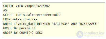
The subquery that will be used will represent a list of the top three salespeople for a single quarter based on the number of invoices. For simplicity in the example queries, this subquery will be saved as a view. For a query as simple as this, there is probably no performance difference between using a view-based SQL, a CTE-based SQL, or a traditional subquery.
The IN operator can be used to find rows in a query where one column can be matched against a value in a list of values. The list of values can be hard-coded as a comma-separated list, or it can come from a subquery, as in this example.
IN statements are easy to write and understand. The only drawback is that they can only compare a single column from the subquery to a single column from the main query. If it is necessary to compare 2 or more values, the IN operator cannot be used.
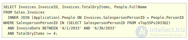
Below is a query that returns some invoices belonging to our top group of salespeople. Note that the subquery returns exactly one row. This is a requirement for using the IN operator. Also note that the query in parentheses is itself a fully functional query on its own. It can be selected and executed by itself.
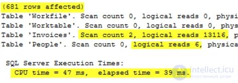
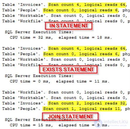
This information is output when this query is executed with the STATISTICS IO and STATISTICS TIME functions enabled, or with EXPLAIN.
This output will give us some performance metrics to compare with the other options. If you don’t know how to get this output, refer to the EXPLAIN or STATISTICS IO documentation.
The EXISTS operator works similarly to the IN operator, except that it can be used to find rows where one or more columns from the query can be found in another dataset, usually a subquery. Hard-coding is not possible with EXISTS.
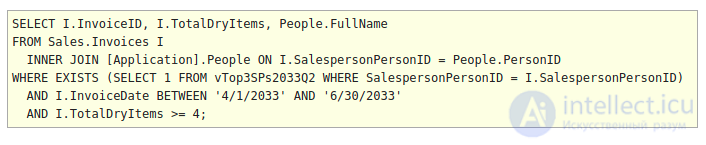
Below is the same query as above, except that IN has been replaced with EXISTS. The format of EXISTS and its subquery is somewhat different from that of IN. In this case, the subquery references the column I.SalespersonPersonID, which appears to be available to the subquery. For this reason, the subquery cannot be executed on its own and can only be executed in the context of the entire query. This can sometimes be difficult to understand.
Logically, you can think of this as running the subquery once for each row in the main query to determine whether the row exists. If the row exists when the subquery is executed, then the returned boolean value is true. Otherwise, it is false. The columns selected in the subquery do not matter, since the result depends only on the existence or absence of a row based on the FROM / JOIN / WHERE clauses in the subquery.
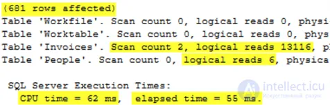
Executing this query returns the following statistical output, which is virtually identical to the IN operator.
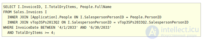
A regular JOIN can be used to find matching values in a subquery. Like EXISTS, JOIN allows one or more columns to be used to find matches. Unlike EXISTS, JOIN is simpler to implement. The downside of JOIN is that if there are any duplicate rows in the subquery based on the JOIN predicate, then the main query will duplicate rows, which can lead to incorrect query conclusions. Both IN and EXISTS ignore duplicate values in the subquery. Take special precautions when joining tables this way. In this example, the view will not return duplicate SalespersonPersonID values, so this is a safe implementation of JOIN.
Executing this query returns the following statistical output, which, again, is virtually identical to the IN and EXISTS versions of the query.
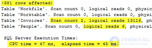
The statistics for each of these three options are virtually identical because the optimizer merges all 3 options into the same query plan. This can be verified by running all three queries together while viewing the actual execution plans. The screenshot below shows a single plan, but the same plan is displayed for each of the three query variants.

Each copy of the query plan shows a missing index recommendation. Implementing this recommendation and creating the index will change the query plans and performance statistics. Will it change them all the same way? Let’s find out. First, create the index, then re-run the 3 queries.
Now run all 3 statements together again. Something interesting happens. All 3 plans changed compared to the versions before the index was created, but this time they are not identical. IN and EXISTS have the same new plan, but JOIN has a different plan.
The plan for IN and EXISTS used the new index twice and performed a seek on the People table.

This plan was produced for the JOIN version of the query. It used the new index twice, but performed a scan of the People table.
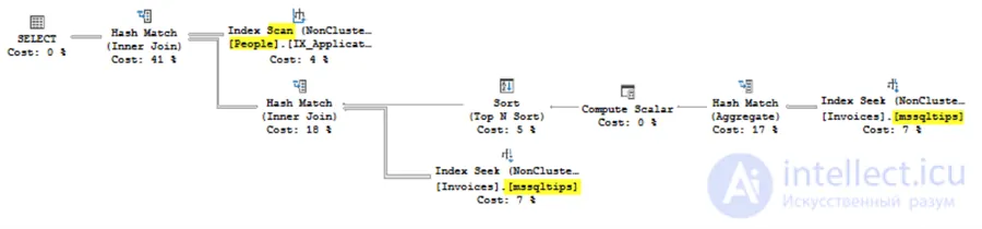
Checking the I/O and time statistics for the 3 queries shows identical statistics for the 2 queries with a shared plan, but improved statistics and execution time for the JOIN version. If this were a query being prepared for promotion to production, then JOIN would probably be the best option.
This query is an excellent example of the fact that, although the optimizer strives to treat all options the same way, it does not always do so. Using this performance-testing methodology, along with an understanding of the value and limitations of each query option, will allow a developer to make the best choice in each situation.


Comments