
Lecture
The QR algorithm is a numerical method in linear algebra for solving the complete eigenvalue problem, that is, for finding all the eigenvalues and eigenvectors of a matrix. It was developed in the late 1950s independently by V. N. Kublanovskaya and J. G. F. Francis.
The QR algorithm was preceded by the LR algorithm, based on LU decomposition. The QR algorithm is more stable than the LR algorithm and so has displaced it; the LR algorithm is little used today. It was, however, the first step toward the modern QR methods.
The LR algorithm was developed in the early 1950s by Heinz Rutishauser, who worked as an assistant to Eduard Stiefel at the Swiss Federal Institute of Technology (ETH) in Zurich. Stiefel suggested that Rutishauser use the sequence of moments u 0 T A k x 0 , k = 0, 1, ... (where x 0 and u 0 are arbitrary vectors) to find the eigenvalues of A . Rutishauser used Alexander Aitken's algorithm for this task and developed it into the quotient-difference algorithm (qd algorithm for short), from which the term qd algorithm derives.
After formulating it in a computationally suitable way, he discovered that the algorithm was in fact an iteration A k = L k U k ( LU decomposition ), A k +1 = U k L k , applied to a tridiagonal matrix, from which the algorithm derives LR
Let A be a real matrix for which we want to find the eigenvalues and eigenvectors. Set A0=A. At the k-th step (starting from k = 0) we compute the QR decomposition Ak=QkRk, where Qk is an orthogonal matrix (that is, QkT = Qk−1), and Rk is an upper triangular matrix. We then define Ak+1 = RkQk.
Note that

that is, all the matrices Ak are similar, so their eigenvalues are equal.
Let all the leading principal minors of the matrix A be nondegenerate. Then the sequence of matrices Ak as  converges in form to a block upper triangular form, corresponding to blocks with eigenvalues equal in absolute value.
To obtain the eigenvectors of the matrix, one must multiply together all the matrices Qk.
The algorithm is considered computationally stable, since it proceeds by orthogonal similarity transformations.
Let us assume that the eigenvalues of the positive-definite matrix A are ordered by decreasing magnitude:

Let

and let S be the matrix composed of the eigenvectors of the matrix A. Then the matrix A can be written as a spectral decomposition

Let us find an expression for the powers of the original matrix in terms of the matrices Qk and Rk. On the one hand, by definition of the QR algorithm:

Applying this relation recursively, we obtain:

Introducing the following notation:


we obtain

On the other hand:

Equating the right-hand sides of the last two formulas, we obtain:

Suppose that an LU decomposition of the matrix ST exists:

then

Multiplying on the right by the inverse of U, and then by the inverse of Λk:


It can be shown that

As  , without loss of generality we may assume that the diagonal of the matrix L consists of ones, so that

Let us denote

where the matrix Pk is upper triangular, being a product of upper triangular and diagonal matrices.
Thus we have proved that
 .
.
From the uniqueness of the QR decomposition it follows that if the product of an orthogonal matrix and a triangular matrix converges to an orthogonal matrix, then the triangular matrix converges to the identity matrix. It follows that

That is, the matrices Sk converge to the matrix of eigenvectors of the matrix A.
Since

then

Passing to the limit, we obtain:

Thus we have proved that the QR algorithm solves the complete eigenvalue problem for a symmetric positive-definite matrix.
Under certain conditions the sequence of matrices  converges to a triangular matrix, the Schur decomposition of the matrix
  . In this case the eigenvalues of the triangular matrix lie on its diagonal, and the problem of finding the eigenvalues is considered solved. In convergence tests it is not practical to require exact zeros in the zero part of the matrix, but one can use Gershgorin's circle theorem[en], which sets bounds on the errors.
In its original state (without any additional transformations) the matrix makes each iteration comparatively expensive. The cost of the algorithm can be reduced by first reducing the matrix to upper Hessenberg form (the cost of obtaining which, by the method based on the Householder transformation, is estimated at 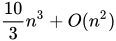 arithmetic operations), and then using a finite sequence of orthogonal similarity transformations. This algorithm is somewhat similar to a two-sided QR decomposition. (In an ordinary QR decomposition the Householder reflection matrix is multiplied into the original matrix from the left only, whereas when using Hessenberg form the reflection matrix is multiplied into the original matrix from both the left and the right.) Finding the QR decomposition of an upper Hessenberg matrix is estimated at
  arithmetic operations. Because the Hessenberg form is almost upper triangular (it has only one nonzero subdiagonal element), the number of iterations required for the QR algorithm to converge can be reduced significantly.
If the original matrix is symmetric, the upper Hessenberg matrix is also symmetric and therefore tridiagonal. The entire sequence of matrices has this same property. In this case the cost of the procedure is estimated at 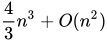 arithmetic operations using the method based on the Householder transformation. Finding the QR decomposition of a symmetric tridiagonal matrix is estimated at
  operations.
The rate of convergence depends on the degree of separation of the eigenvalues, and in practical implementations “shifts” are used, explicitly or implicitly, to increase the separation of the eigenvalues and speed up convergence. In the typical case for symmetric matrices, the QR algorithm finds one eigenvalue exactly (reducing the dimension of the matrix) in one or two iterations, which makes this approach both efficient and reliable.
In modern computational practice the QR algorithm is implemented using its implicit version, which simplifies the addition of multiple “shifts”. Initially the matrix is reduced to upper Hessenberg form 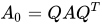 , just as in the explicit version. Then, at each step the first column of is transformed, via a small-dimensional Householder similarity transformation, into the first column of
  (or
(or  ), where is a polynomial of degree
  that determines the “shift” strategy (usually
  , where
  and
and  are the two eigenvalues of the trailing 2×2 submatrix of , the so-called implicit double shift). Then successive Householder transformations of size
  are carried out in order to bring the working matrix back to upper Hessenberg form.
Let  be chosen. Then the procedure can be written in short as the QR decomposition
 followed by re-forming
  , the multiplication being carried out in reverse order. This procedure is a direct generalization of the simultaneous power method for determining the first
  eigenvalues of the matrix. This connection is derived from subspace iteration. The simultaneous inverse power method is likewise carried out indirectly.
Let  be set. This means that, as an alternative, the method can also be written as the QR decomposition
 followed by re-forming, together with the shift correction,
  as shown. Usually the shift
 is chosen so as to approximate the smallest eigenvalue. The last diagonal element can be used
 for this purpose. The simple QR iteration is the result of setting all shifts to zero.
If has Hessenberg form, then so must
  , since as a product of a matrix with a subdiagonal and a matrix without one it likewise has Hessenberg form; the same applies to. Thus, once the matrix in the QR algorithm has been reduced
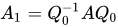 to Hessenberg form, this form is preserved throughout the entire algorithm.
A symmetric real matrix  has only real eigenvalues. Symmetry is preserved in all of them during the operation of the QR algorithm. For symmetric matrices, Wilkinson (1965) proposed that the eigenvalue of the lower-right
 submatrix
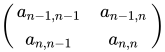
that lies closer to  be chosen as the shift. Wilkinson showed that the matrix sequence thus defined
 converges to a diagonal matrix whose diagonal elements are the eigenvalues
  . The rate of convergence is quadratic.
A pair of simple shifts can be combined into a single iteration step. As a consequence, this means that for real matrices one can dispense with complex shifts. In the notation introduced above

The QR decomposition for the quadratic polynomial  , is estimated at
  . The coefficients of this polynomial are real even for a conjugate pair of complex shifts. Thus the complex eigenvalues of real matrices can also be approximated without using complex numbers in the computation.
The usual choice for this double shift consists of the eigenvalues of the lower-right submatrix, i.e. the quadratic polynomial is the characteristic polynomial of this block,
 .
.
Let a number  greater than
  but much smaller than the size
  of the matrix be chosen. The polynomial
 can be regarded as the characteristic polynomial of the lower-right
  submatrix of the current matrix to be used for the shift. Another strategy is to use the
 eigenvalues of the lower-right
  submatrix to be determined, together with of the smallest eigenvalues
  chosen below. With these, the QR decomposition
 as well as
follows directly.
With repeated shifting it is often found that the lower-left  blocks in the sequence of iterated matrices become small particularly quickly, and thus the eigenvalue problem is split (deflated).
Combining several shifts in the general form is very time-consuming. As mentioned above, the effort can be reduced by, at the preparatory stage, reducing to Hessenberg form. Since each multi-shift step can consist of individual (even complex) shifts, the Hessenberg form is preserved throughout the entire algorithm.
This makes it possible to turn the QR algorithm into the “bulge-chasing” algorithm, which creates a bulge in the Hessenberg form at the upper end of the diagonal, then “chases” it down the diagonal, and finally pushes it out of the matrix at the lower end. .
 do
do using one of the variants described above,
 .
. with respect to the first unit vector. Since in only the first
  components are nonzero, this reflection has a simple block form.
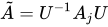 and transform it so that
  is returned to Hessenberg form.
We obtain  consisting of the products
  , so let these blocks be of the diagonal form
  .
.

Comments