
Lecture
The Adams method is a finite-difference multistep method for the numerical integration of first-order ordinary differential equations. Unlike the Runge–Kutta method, it uses not one but several values already computed at previous points to calculate the next value of the sought solution.
It is named after the English astronomer John C. Adams, who proposed it in 1855.
Let a system of first-order differential equations be given
 ,
,
for which a solution must be found on a grid with constant step  . The computational formulas of the Adams method for solving this system have the form:
a) extrapolating — the Adams–Bashforth method
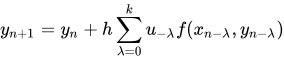 ,
,
b) interpolating, or implicit — the Adams–Moulton method
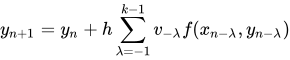 ,
,
where  are certain computable constants.
For the same  , formula b) is more accurate , but it requires solving a nonlinear system of equations to find the value
  . In practice, an approximation is found from a), and then one or more refinements are carried out using the formula
 .
.
Adams methods of order require the solution to be computed in advance at initial points. To compute the initial values, one-step methods are usually used, for example the 4-stage Runge–Kutta method of 4th order accuracy.
The local error of Adams methods of order is  . The structure of the error of the Adams method is such that the error remains bounded, or grows very slowly, in the case of asymptotically stable solutions of the equation. This makes it possible to use this method for finding stable periodic solutions, in particular for computing the motion of celestial bodies.
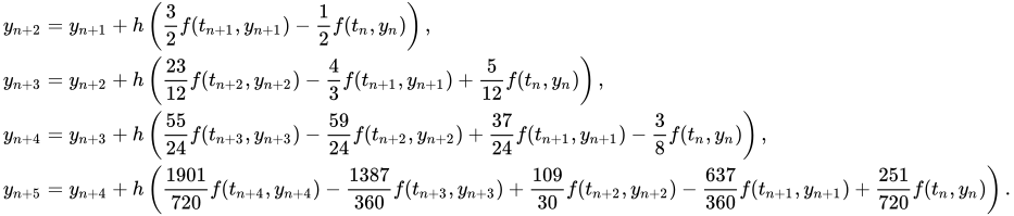
Explicit Adams–Bashforth methods
 , (Euler's method)
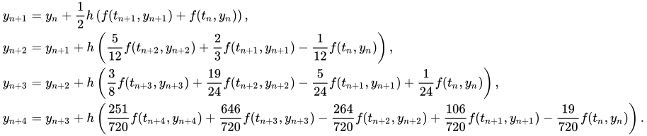
Implicit Adams–Moulton methods
 , (implicit Euler method)
Implementation of the Adams method in the C language..
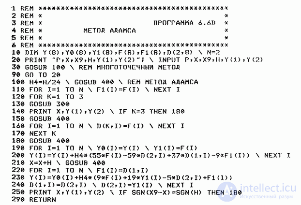
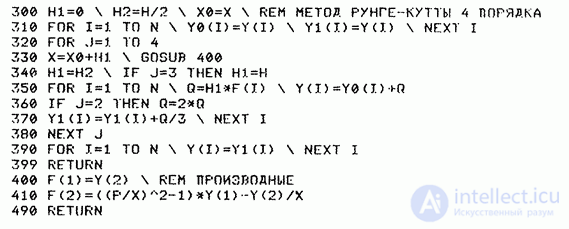
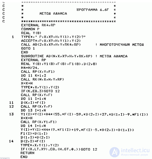
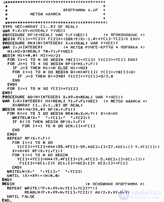
To start the extrapolating Adams method, 4 initial values of the function are required. One value is already given, while the remaining ones are obtained by the 4th-order Runge–Kutta method. After the value at the end of the interval has been computed, the relative error is computed (from the current and previously obtained values of the function with step h) and compared with the specified value. If the resulting error is smaller than the specified one, the task is considered complete and control returns to the calling program together with the obtained value of the function. If not, the step is halved and the entire process, starting from the Runge–Kutta method, is repeated again (to compute new values of the function). This continues until the resulting error becomes smaller than the specified one.
For the program to work, a function is needed that computes the right-hand sides of the system of differential equations. This is the function func (double *y, double *ys, double x). Since the problem requires solving the equation y(3)+2y’’+3y’+y=5+x2, we form a system of first-order differential equations. It looks like this:

Each time the left-hand sides of this system are computed, y, y’ and y’’ are differentiated, i.e. the new values of y’, y’’, y’’’ are computed accordingly.
Well, if we put all this into a C program, we get the function func (see listing 17 of the problem).
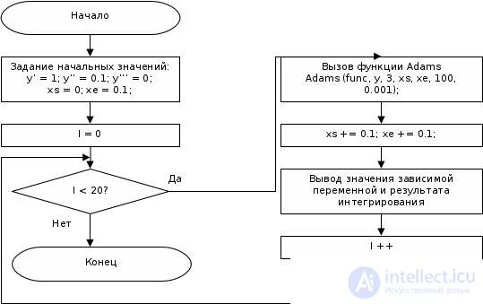
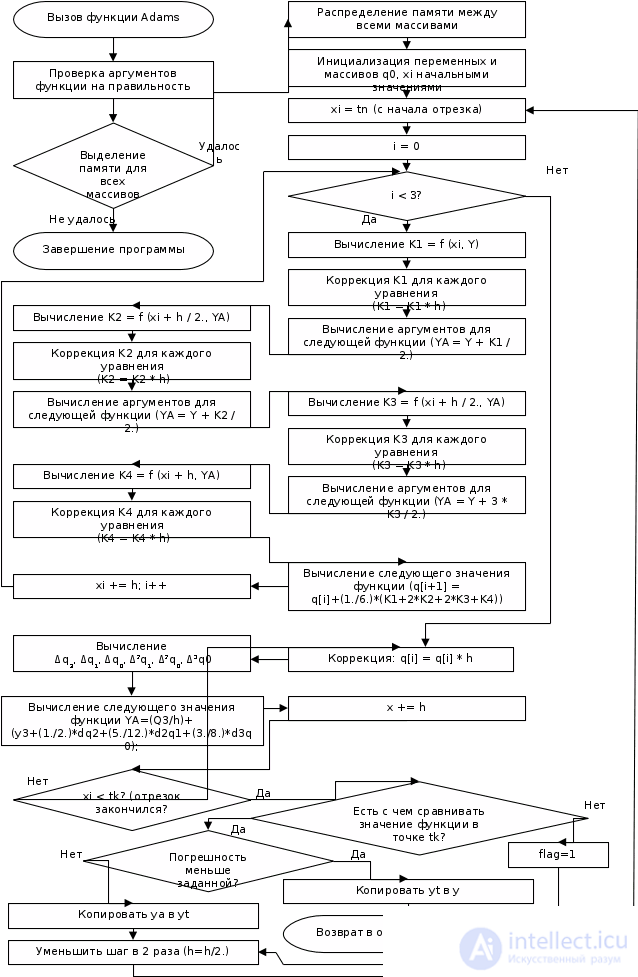
// Problem 17. Numerical integration of a system of differential equations
// by the Adams method. The program is intended for compilation with Micro$oft C 6.00
// or Borland C 3.1+
// (C) 2004 REPNZ. All rights reserved. Release date is 2.04.2004
#include
#include
#include
void func (double *y, double *ys, double t)
{ // function computing the right-hand sides of the equations
ys = y ; // ys is the first derivative; ys is the second, etc.
ys = y ; // t is the independent argument
ys = 5 + t * t - y - 3. * y - 2. * y ;
}
void Adams (
void f (double *y, double *ys, double x),
// Function that computes the right-hand sides of the system
double *y, // Array of size n holding the values of the dependent variables
int n, // Array of size n holding the values of the derivatives
double tn, // Start of the integration interval
double tk, // End of the integration interval
int m, // Initial number of subdivisions of the integration interval
double eps) // Relative integration error
{
double *k1, *k2, *k3, *k4; // For the Runge-Kutta method
double *q0, *q1, *q2, *q3; // Derivative values for the Adams method
double *ya; // Temporary array
double *y0, *y1, *y2, *y3; // Function values for the Adams method
double h; // Integration step
double xi; // Current value of the independent variable
double eps2; // For error estimation
double dq2, dq1, dq0, d2q1, d2q0, d3q0; // increments
int flag = 0; // 0, while the first computation is underway
int i, j; // Indices
if (m < 4) m = 4; // Minimum 4 segments
if (tn >= tk)
{ printf ("\nInvalid arguments\n");
abort (); // Invalid arguments
}
// Allocate memory for the variable arrays
if ((k1 = malloc ((4 + 4 + 4 + 1) * n * sizeof (double))) == 0)
{ printf ("\nMemory allocation error\n");
abort (); // Abort if unsuccessful
}
// Distribute the memory among the arrays:
// For the 4th-order Runge-Kutta method
k2 = k1 + n; k3 = k2 + n; k4 = k3 + n;
// 4 previous values of the function
y0 = k4 + n; y1 = y0 + n; y2 = y1 + n; y3 = y2 + n;
// For the temporary data-collection array
ya = y3 + n;
// For the Adams method
q0 = ya + n; q1 = q0 + n; q2 = q1 + n; q3 = q2 + n;
h = (tk - tn) / m; // Step
eps = fabs (eps); // Absolute value of the error
start: // Computation starts here
xi = tn; // Start of the interval
// Compute the function values y0...y3, i.e. y[i-3] ... y
// The first value of the system of equations is already given: y ...
///////////////////////////////////////////////////////////////////////
// - 4th-order Runge-Kutta method - //
///////////////////////////////////////////////////////////////////////
for (j = 0; j < n; j++) y0[j] = y[j]; // Copy it into y0
f (y0, q0, xi); // Fill q0, based on the values from y0
for (j = 0; j < n; j++) q0[j] *= h; // Form q0
xi += h; // Next step
// ... and the remaining 3 are obtained using the 4th-order Runge-Kutta method.
for (i = 0; i < 3; i++) // i - WHICH VALUE ALREADY EXISTS
{ // AND WE COMPUTE THE VALUES Y[i+1]!!!!
// First we need the coefficients k1
// Element y[i, j] = y0 + (i * n) + j = y0[i * n + j]
f (&y0[i * n], k1, xi); // Compute f(xi, yi) = k1 / h
// And for each differential equation of the system we carry out
// the operations of computing k1, and also prepare in ya the argument for
// computing k2
for (j = 0; j < n; j++)
{
k1[j] *= h; // Finally compute k1
ya[j] = y0[i*n+j] + k1[j] / 2.;
// And one of the arguments for the function
} // computing k2
f (ya, k2, xi + (h / 2.)); // Compute f(xi,yi) = k2 / h
for (j = 0; j < n; j++)
{ // Finally compute k2
k2[j] *= h;
ya[j] = y0[i*n+j] + k2[j] / 2.; // And one of the arguments for the function
} // computing k3
f (ya, k3, xi + h / 2.); // Compute f(xi,yi) = k3 / h
for (j = 0; j < n; j++)
{
k3[j] *= h; // Finally compute k3
ya[j] = y0[i*n+j] + k3[j]; // And one of the arguments for the function
} // computing k4
f (ya, k4, xi + h); // Compute f(xi,yi) = k4 / h
for (j = 0; j < n; j++) k4[j] *= h; // Finally compute k4
// We need to compute the increment of each of the n functions
for (j = 0; j < n; j++) // Compute the next value
// of the function
// Y[i+1] = Yi + ...
y0[(i+1)*n+j] = y0[i*n+j] + (k1[j] + 2. * k2[j] + 2 * k3[j] + k4[j]) / 6.;
// And the new value q[i+1]
f (&y0[(i+1)*n], &q0[(i+1)*n], xi); // qi = f (xi, yi);
for (j = 0; j < n; j++) q0[((i+1)*n)+j] *= h;
xi += h; // Next step }
///////////////////////////////////////////////////////////////////////
// - Adams method - //
///////////////////////////////////////////////////////////////////////
// So, the first 4 values have been computed. This is enough to begin the Adams
// method for step h.
// In y0...y3 lie 4 function values (_NOT_DERIVATIVES!!!).
// And in q0...q3 lie the values of the _derivatives_ of these functions, multiplied by h
// q0..q3, and also y0..y3, form queues with 4 elements
again: // Compute the new value of the function Yi (this is Y[i+1])
for (j = 0; j < n; j++)
{ // All the increments
dq2 = q3[j] - q2[j]; dq1 = q2[j] - q1[j]; dq0 = q1[j] - q0[j];
d2q1 = dq2 - dq1; d2q0 = dq1 - dq0;
d3q0 = d2q1 - d2q0;
// the new function value (in ya for now)
ya[j] = y3[j] + (q3[j] + (dq2 / 2.) + (5. * d2q1 / 12.) + (3. * d3q0 / 8.));
// Shift all the arrays forward by 1 and add to the queue the new
// function value
y0[j] = y1[j]; y1[j] = y2[j]; y2[j] = y3[j]; y3[j] = ya[j];
// Just shift q, without adding anything yet
q0[j] = q1[j]; q1[j] = q2[j]; q2[j] = q3[j];
}
// Put the new value into the queue as q3
f (y3, q3, xi); // q3 = f (xi, y3);
for (j = 0; j < n; j++) q3[j] *= h; // Compute q3
// The next function value has been computed. Next step
xi += h;
// Continue integrating?
if (xi < tk) goto again; // Yes.
// If this is the first time here, recompute once more with step h/2
if (flag == 0)
flag = 1; // There will now be something to compare against
else
{
// Not the first time - estimate the error
// y3 now holds the value of the just-computed function,
// and y2 holds the value of the function computed with step h * 2
// relative to the current one
for (j = 0; j < n; j++)
{ eps2 = fabs (((y3[j] - y2[j]) / y2[j]));
if (eps2 > eps) break; // If the error is too large
}
if (j == n) // If everything is OK
{ // Copy the result
for (j = 0; j < n; j++) y[j] = y3[j];
free (k1); // Free the memory
return; // Return to main
}
}
// For some reason we did not exit the function -
// so we halve the step and repeat
// everything, starting from the Runge-Kutta method
h /= 2.; // Halve the step
goto start; // Repeat the computation from the start, with the new parameters
}
int main ()
{
double y , xs, xe;
int i;
y = 1.; y = 0.1; y = 0.; // Initial conditions
xs = .0; xe = .1; // Start of integration
printf ("x = %5.3lg, y(%4.2lg) = %10.3lg\n", xs, xs, y );
for (i = 0; i < 20; i++)
{
Adams (func, y, 3, xs, xe, 10, 1.e-3);
xs += 0.1; xe += 0.1;
printf ("x = %5.3lg, y(%4.2lg) = %10.3lg\n", xs, xs, y );
}
return 0;
}

Comments