
Lecture
Short-time Fourier transform — is a variant of the Fourier transform, defined as follows:
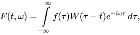
where  — is some window function. In the case of the discrete transform, the window function is used in a similar way:

There are many mathematical formulas that visually improve the frequency spectrum at the boundary discontinuities of the window. For this purpose the following are used: the triangular (Bartlett) window, the sine window, the sine-cubed window, the sine-to-the-4th-power window, the Parzen window, the Welch window, the Gaussian window, the Hann window, the raised-cosine (Hamming) window, the Dolph–Chebyshev window, the window with ripple, the Rosenfeld window, the Blackman–Harris window, the horizontal window, and the flat-top window. There is also a technique for the mutual overlap of windows, in which it is usually possible to choose how many samples from the previous window will be averaged with the current window.
In practice it is not possible to obtain a signal over an infinite interval, since there is no way to know what the signal was before the device was switched on or what it will be in the future. Limiting the analysis interval is equivalent to multiplying the original signal by a rectangular window function. Thus, the result of the short-time Fourier transform is not the spectrum of the original signal, but the spectrum of the product of the signal and the window function. The result is an effect known as spectral leakage. The danger is that the side lobes of a signal of higher amplitude can mask the presence of other signals of lower amplitude.
To combat spectral leakage, a smoother window function is used, whose spectrum has a wider main lobe and a lower level of side lobes. The spectrum obtained by means of the short-time Fourier transform is the convolution of the spectrum of the original ideal signal and the spectrum of the window function.
The distortions introduced by the use of windows are determined by the size of the window and its shape. The following main properties of window functions are distinguished: the width of the main lobe at the -3 dB level, the width of the main lobe at the zero level, the maximum level of the side lobes, and the attenuation coefficient of the window function.
The short-time Fourier transform is used in communications for the synthesis of frequency filters, for example, in the frequency-division multiplexing method with multiple carriers, using a filter bank (comb) of frequency filters, FBMC .
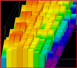
STFT is used for analyzing an audio signal over time.
STFT, as well as standard Fourier transforms and other tools, are often used for analyzing music. A spectrogram can, for example, display frequency on the horizontal axis: the lowest frequencies on the left, and the highest on the right. The height of each band (supplemented by color) represents the amplitude of the frequencies in that range. The depth dimension represents time, with each new column representing a separate transform. Audio engineers use this kind of visualization to obtain information about an audio sample, for example, to identify the frequencies of certain noises (especially when using a higher frequency resolution), or to find frequencies that may be more or less resonant in the space where the signal was recorded. This information can be used for equalization or for adjusting other sound effects.
| Method | Complexity |
|---|---|
| Direct implementation | O(TF) |
| FFT-based | O(TN log2N)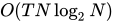 |
| Recursive | O(TF) |
| Chirp Z-transform | O(TN log2N) |
When using the short-time Fourier transform it is not possible to simultaneously provide good resolution in both time and frequency. The narrower the window, the higher the time resolution and the lower the frequency resolution.
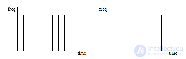
Comparison of the short-time Fourier transform with different windows. On the left (narrow window) — good time resolution, on the right (wider window) — good frequency resolution.
The resolution along the axes is constant. This is undesirable for a number of tasks in which information across frequencies is distributed unevenly. In such tasks, the wavelet transform can be used as an alternative to the short-time Fourier transform; its time resolution increases with frequency (while the frequency resolution decreases).

Rectangular window; B=1.00
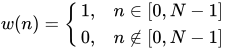
Obtained automatically when the sample is limited to N samples. Maximum level of the side lobes of the frequency response: -13 dB.
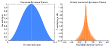
Hann window; B = 1.50

where N — is the window width. Level of side lobes: −31.5 dB.
Hamming window

Level of side lobes: -42 dB.
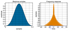
Blackman window; α = 0.16; B=1.73


Level of side lobes: -58 dB (α=0.16).
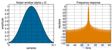
Kaiser window, α =2; B=1.5
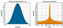
Kaiser window, α =3; B=1.8
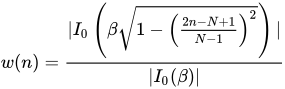
where 0 — is the modified Bessel function of the first kind, order zero;
  — is a coefficient determining the fraction of energy concentrated in the main lobe of the window function's spectrum. The larger is, the greater the fraction of energy, the wider the main lobe, and the lower the level of side lobes. In practice, values from 4 to 9 are used.
For the short-time Fourier transform in digital form, it is possible to apply not only the weighting of each digital sample in the process of forming the convolution, but also the equivalent weighted summation of the responses of the Fourier transform .
For example, weighting with the Hann window (Hanning) and the Hamming window can be represented as:
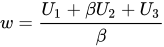 ,
,
where  ,
,  ,
,  - are the original responses of the Fourier transform,
  - is the result of the windowed transform,
  corresponds to the Hann window (Hanning),
  - to the Hamming window .
The implementation of this weighting is carried out in a sliding-window mode over the array of responses of the Fourier transform.

Comments