
Lecture
Reversible computing (English: Reversible computing) — a model of computation in which the computational process is, to some degree, reversible. For example, in a computational model that uses sets of states and transitions between them, a necessary condition for reversibility of computation is the possibility of constructing a single-valued (injective) mapping of each state onto the one that follows it. Throughout the 20th century and the early 21st century, reversible computing has generally been classed among the unconventional models of computation.
There are two main types of reversibility of computation: physically reversible and logically reversible.
A process is physically reversible if, by its completion, the system has not increased its physical entropy, that is, the process is isentropic. Physically reversible circuits include: charge-recovery logic (charge-conserving logic), adiabatic circuits, adiabatic computing. In practice, a non-stationary physical process cannot be fully physically reversible (isentropic), though for well-isolated systems an approximation to complete reversibility is possible.
Probably the greatest incentive for studying technologies for implementing reversible computing is that they appear to be the only way to improve the energy efficiency of computation beyond the fundamental limits predicted by the Neumann–Landauer principle , according to which at least kT ln(2) of heat (about 3×10⁻²¹ J at T=300K) is dissipated for every irreversible operation on a bit (upon erasure of a bit of information). At the start of the 21st century, computers dissipated roughly a million times more heat than this; by the start of the 2010s the difference had fallen to a few thousand .
As was shown by Rolf Landauer (English) of IBM in 1961 , for a computational process to be physically reversible, it is also required to be logically reversible (logically reversible). In Landauer's principle he was the first to formulate the rule according to which erasing N bits of unknown information is always accompanied by an increase in thermodynamic entropy of at least Nk ln(2). A discrete deterministic computational process is called logically reversible if the transition function mapping the old state of the system to the new one is injective (each new state corresponds uniquely to one old state), that is, if the input logical state of the circuit can be determined from information about its final logical state.
For non-deterministic (probabilistic or random) processes, physical reversibility can be achieved under less strict constraints, namely under the condition that the total set of all possible initial states does not decrease (on average) over the course of the computation.
One of the first proposals for implementing reversible computing was put forward in the work of Charles Bennett (English)Russian, (IBM Research, 1973). A great many researchers have since proposed dozens of concepts for reversible computing, including reversible logic gates, electronic circuits, processor architectures, programming languages, and algorithms .
For implementations of reversible computing circuits, and for evaluating their complexity and constraints, a formalisation through reversible gates — analogues of logic gates — is used. For example, the NOT (inverter) gate is reversible, since it preserves information. At the same time, the exclusive OR (XOR) logic gate is irreversible — the values of its inputs cannot be recovered from the single output value. A reversible analogue of XOR can be the controlled-NOT gate (CNOT — controlled NOT).
Reversible gates can be useful for solving the problem of heat dissipation in future generations of processors, and they are closely connected with the theory of quantum computing. The topic is also interesting in its own right. A great deal has been written about it, including in the references given above, so I will try not to dwell too much on things that are already fairly well known.
Put very simply, a gate is reversible when the values on its inputs can always be recovered from the values on its outputs. For working with binary data, the universal Toffoli or Fredkin gates are usually used. Both gates have three inputs and three outputs, since, unlike the irreversible case, it is not possible to build a set for performing an arbitrary operation on data out of reversible binary gates with two inputs.
Nation uses a set of three elements to describe it, denoted by the symbols R, P, S, which correspond to the first letters of the English words for rock, scissors and paper. The game “rock, paper, scissors” (which has also been written about here more than once) is also known in Hawaii as “jan-ken”. Under the rules of the game, one of the three objects beats another based on a cyclic set of preferences. This is usually depicted on a circular diagram, but it can also be written in a line:
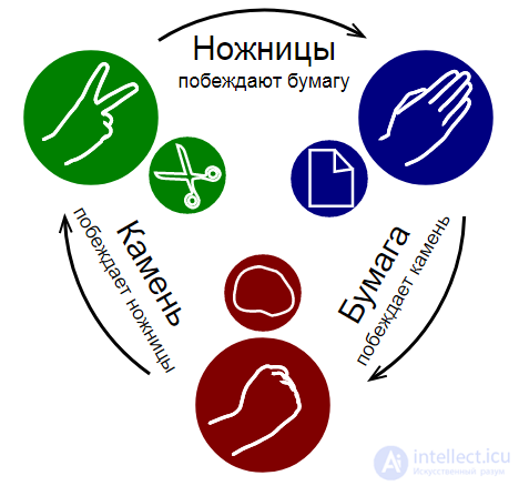
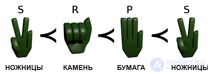
The mathematical symbol for the relation “precedes” (Unicode 227A) used in the picture is missing from many fonts, so in the text it has been replaced with < —
How is this related to logic? It is known that if we set FALSE=0, TRUE=1, then “AND” corresponds to the “minimum” function, and “OR” to the “maximum” function. The same trick is used in multi-valued and fuzzy logic, since with such a definition many properties of ordinary logic hold automatically. So, specifying the relations between elements defines analogues of logical operations. True, with a cyclic set of preferences among three elements, some properties have to be sacrificed. What can you do, it is a different logic.
The table for the analogue of “OR” under this approach looks like this
| Alternative OR | R | P | S |
| R | R | P | R |
| P | P | P | S |
| S | R | S | S |
The table for the “AND” operation is built similarly
| Alternative AND | R | P | S |
| R | R | R | S |
| P | R | P | P |
| S | S | P | S |
Let us try to imagine a reversible analogue of the ordinary “OR” gate. Suppose it has two inputs (and two outputs, since it must be reversible), binary values are fed to the inputs, and one of the outputs must give the result of the “OR” operation. It turns out that the same value of 1 (TRUE) on this output can arise from three different input combinations: 11, 01, 10. If the second output could take three different values, this could be used to make such a gate reversible.
So, already fairly simple estimates lead to the idea of using a ternary system on at least one output. But what if we try working with three values on all inputs and outputs – can a reversible gate be obtained if we use ternary logic?
A fairly common choice is Łukasiewicz ternary logic. It can also be built using the max/min trick mentioned above, if we assume that the third value corresponds to some number x, 0 < x < 1, for example x = 1/2. This gives the well-known ternary tables, for “OR”:
| “Ternary OR” | 0 | x | 1 |
| 0 | 0 | x | 1 |
| x | x | x | 1 |
| 1 | 1 | 1 | 1 |
For “AND”:
| “Ternary AND” | 0 | x | 1 |
| 0 | 0 | 0 | 0 |
| x | 0 | x | x |
| 1 | 0 | x | 1 |
Suppose again that we have a ternary gate with two inputs and two outputs. One of the functions given above is fed to the first output. Can we choose a function for the second output so that the gate is reversible? It turns out that we cannot. The reason is that for an arbitrary reversible function in a 3×3 table describing any input, every value must occur exactly three times.
Indeed, nine possible pairs of values can be fed to the input
00 01 0x 10 11 1x x0 x1 xx
and since the gate is reversible, each of these nine pairs must also appear at the output for one of the combinations at the input. It can be seen that in these pairs, any value of the first (and second) element occurs exactly three times.
That is, three zeros, three ones, three x's. But instead, in the table for ternary “OR” there is only one zero and five ones. In the second table, for “AND”, it is the opposite — five zeros and one one, which also does not work.
So, although reversible ternary gates on their own, and ternary logic on its own, are both fairly widely used, it is difficult to reconcile the two together. This is where the “alien” logic comes to the rescue. For clarity, let us replace R,P,S with 0,1,$.
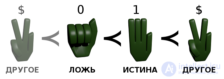
Here is the table for “OR”
| “Alternative OR” | 0 | 1 | $ |
| 0 | 0 | 1 | 0 |
| 1 | 1 | 1 | $ |
| $ | 0 | $ | $ |
For the values 0, 1, it coincides with ordinary “OR”, but at the same time it has the property already mentioned, needed to create a reversible ternary gate (each value occurs exactly three times). The situation with the table for the “AND” operation is similar
| “Alternative AND” | 0 | 1 | $ |
| 0 | 0 | 0 | $ |
| 1 | 0 | 1 | 1 |
| $ | $ | 1 | $ |
Now, to build a complete version of the reversible ternary gates, we still need to choose a table for the second, auxiliary output. In ordinary arithmetic, to invert the function max(a,b), the second output could use b–a. Something similar can be used in our example
| “Alternative difference” | 0 | 1 | $ |
| 0 | 0 | $ | 1 |
| 1 | 1 | 0 | $ |
| $ | $ | 1 | 0 |
It fits – here is what the complete ternary reversible “OR” gate looks like
| Input | 00 | 01 | 0$ | 10 | 11 | 1$ | $0 | $1 | $$ |
| Output | 00 | 11 | 0$ | 1$ | 10 | $1 | 01 | $$ | $0 |
It can be seen that each of the nine possible combinations occurs exactly once at the output, so the operation is reversible. The action of this gate can also be described as follows: it leaves the pairs 00, 0$ unchanged, cyclically permuting seven pairs (01, 11, 10, 1$, $1, $$, $0)
So, applying the gate seven times will leave any pair of values unchanged, and the inverse operation corresponds to applying six gates in a row. With the Toffoli and Fredkin gates it is simpler, each of them coincides with its own inverse.
If only the values zero and one are fed to the input, this ternary gate implements the ordinary logical “OR” operation. By setting the second input to one, the second output can be used as a “NOT” of the first input. In addition, the gate implements a “fan-out” operation for the binary value fed to the second input, if zero is fed to the first. So this reversible ternary gate is universal for working with binary data.
An example of a reversible ternary “AND” gate is similar
| Input | 00 | 01 | 0$ | 10 | 11 | 1$ | $0 | $1 | $$ |
| Output | 00 | 01 | $$ | 0$ | 10 | 11 | $1 | 1$ | $0 |
This gate leaves the pairs 00 and 01 unchanged, cyclically permuting the pairs
(0$, $$, $0, $1, 1$, 11, 10, 0$)
It too is universal for binary operations, but unlike “OR”, one such gate alone is not enough for “fan-out”. That said, the choice of operation on the second output was fairly arbitrary. The operation on the first input, however, is uniquely determined by three conditions: (1) it must perform the required logical operation for binary data, (2) it must correspond to one of the values at the input, (3) it must not depend on their permutation.
The choice of the second operation is also fairly natural and can be used for other models. Suppose we need to build a reversible gate for Łukasiewicz logic. The problem with this has already been described: some values appear five times in the 3x3 table, whereas they should be equal in number to make a reversible gate.
If we add a lizard and Spock, the same idea can be applied as when extending binary logic to a system of three elements, and given the existing problem of five repetitions in the table for Łukasiewicz ternary logic (0, 1, x), two more elements need to be added ($ and @). Another argument in favour of five values is related to using an analogue of the difference b-a to invert the maximum and minimum: the difference between three integer values from 0 to 2 can take five different values, from -2 to 2.
The relations between the elements can again be depicted on a circular diagram or written in a line
0 <- 1 <- $ <- x <- @ <- 0 <- x <- 1 <- @ <- $ <- 0
The corresponding game is also well known. For example, a version of it was shown in the TV sitcom “The Big Bang Theory” (with a picture explaining it). The correspondences can be chosen as follows: 0 – rock, 1 – paper, $ — scissors, @ — lizard, x – Spock (a native of the planet Vulcan in the “Star Trek” series).
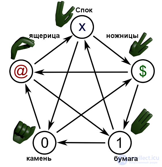
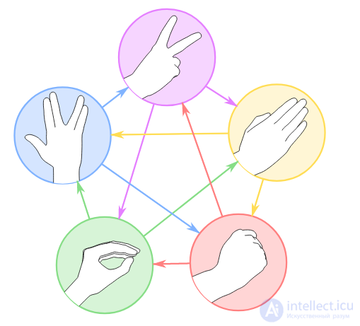
Figure, clockwise from the top: scissors, paper, rock, lizard, Spock
One can go on further; for building similar circular diagrams, sets in which the number of elements is a prime number are especially well suited.
Note that cyclic (collective) logic is not really so “alien”. One of the most characteristic examples is related to the Condorcet and Arrow paradoxes concerning the problem of choice. A typical description of the “voting paradox” can be found in the book by Nobel laureate in economics Kenneth Arrow, “Social Choice and Individual Values”.
Consider a choice among three alternatives (for example, an election with three candidates) A, B, C. Suppose each voter has some ordered system of preferences. That is, if the first alternative is preferred to the second, and the second is preferred to the third, then the first is also preferred to the third. An example of the problems with choice that arise when this criterion is violated is also described below.
Such ordered preferences are an example of transitive relations, and operations with an analogous property are associative, that is, they do not depend on how the brackets are arranged. The definition of the “OR” operation discussed earlier, via specifying relations among elements, fits well with the idea of choice: the operation “A OR B” is simply a choice between A and B, based on some set of preferences (including the case “A OR A”, which, although hard to call a “choice”, also has a perfectly well-defined result, A).
Suppose someone believes that B is better than A, C is better than B (and, by the criterion given earlier, C is better than A). Let us write this choice as
(1) A < B < C
Suppose there are two other ordered sets of preferences
(2) B < C < A
(3) C < A < B
Let us denote the shares of voters with the corresponding set of preferences as P1, P2, P3. Then the share who think B is better than A will be P1+P3, and those who think C is better than B will be P1+P2, but at the same time P2+P3 think A is better than C.
If all the values P1+P2, P2+P3, P1+P3 are greater than half (or, equivalently, any share P1, P2, P3 is less than half), then in voting B beats A, C beats B, but A beats C. A cyclic system of collective preferences is formed, which, to avoid confusion, we denote with the symbol already used for a relation without the property of transitivity
A < — B < — C < — A.
Even if every individual has an ordered set of preferences, without transitivity the collective choice is no longer well-defined. The outcome of the election can depend on the order in which votes are taken and can turn out to be essentially arbitrary. Below are examples of three voting schemes with different orders that lead to the victory of any of the three candidates.
Scheme 1
First round: choice between A and B, B wins
Second round: choice between B (winner of the first round) and C,
C wins (in the second round and in the election)
Scheme 2
First round: choice between B and C, C wins
Second round: choice between C and A, A wins the election
Scheme 3
First round: choice between A and C, A wins
Second round: choice between B and A, B wins the election
The same problem can be illustrated as the absence of associativity in a cyclic system of preferences. Let us denote the choice operation as ||
Then the first two schemes correspond to the following bracket arrangements
((A || B) || C) = B || C = C,
(A || (B || C)) = A || C = A

Comments