
Lecture
In computer engineering, instruction pipelining is a technique for implementing instruction-level parallelism within a single processor. Pipelining aims to keep every part of the processor busy with some instruction by splitting incoming instructions into a sequence of steps (the so-called “pipeline”) carried out by different processor units, so that different parts of several instructions are processed in parallel.
A pipeline is a way of organizing computation used in modern processors and controllers to increase their performance (increasing the number of instructions executed per unit of time — exploiting instruction-level parallelism).
|
Clock cycle
Instr. No.
|
1 | 2 | 3 | +++4 | 5 | 6 | 7 |
|---|---|---|---|---|---|---|---|
| 1 | IF | ID | EX | +++MEM ---- | WB | ||
| 2 | IF | ID | +++EX | MEM | WB | ||
| 3 | IF | +++ID | EX | MEM | WB | ||
| 4 | +++IF | ID | EX | MEM | |||
| 5 | IF | ID | EX | ||||
| (IF = Instruction Fetch, ID = Instruction Decode, EX = Execute, MEM = Memory Access, WB = Register Write Back).
In the fourth clock cycle (the green column), the earliest instruction is at the MEM stage, while the latest instruction has not yet entered the pipeline. |
A pipeline can be partially compared to a queue, but it is incorrect to consider it simply a queue.
Main difference: a queue is a place where data waits to be processed.
task 1
task 2
task 3
   ↓
Worker processes
A pipeline is a sequence of processing stages.
data → step 1 → step 2 → step 3 → result
That is:
Queue = stores and orders tasks
Pipeline = processes data in stages
In a pipelined computer, instructions pass through the central processing unit (CPU) in stages. For example, each step of the von Neumann cycle may have a separate stage: instruction fetch, operand fetch, instruction execution, and result write-back. A pipelined computer usually has “pipeline registers” after each stage. These hold information about the instruction and its computations so that the logic elements of the next stage can carry out the next step.
This scheme allows the processor to complete an instruction every clock cycle. Typically, even-numbered stages operate on one edge of the rectangular clock signal, while odd-numbered stages operate on the other. This provides greater processor throughput than a multi-cycle computer at a given clock frequency, but may increase latency due to the additional overhead of the pipelining process itself. Furthermore, although electronic logic has a fixed maximum speed, the speed of a pipelined computer can be increased or decreased by changing the number of stages in the pipeline. The more stages there are, the less work each stage performs, and consequently the smaller the delays from the logic elements, and the higher its clock frequency can be.
The pipelined computer model often turns out to be the most economical when cost is measured in logic elements per instruction per second. At any given moment, an instruction occupies only one pipeline stage, and on average a pipeline stage is cheaper than a multi-cycle computer. Moreover, with a good implementation, most of the logic in a pipelined computer is used most of the time. By contrast, computers with out-of-order execution typically have a large amount of idle logic at any given moment. Similar calculations usually show that a pipelined computer consumes less energy per instruction.
However, a pipelined computer is usually more complex and more expensive than a comparable multi-cycle computer. As a rule, it has more logic elements, more registers, and a more complex control unit. Likewise, it may consume more energy overall, but less energy per instruction. Processors with out-of-order execution can typically execute more instructions per second, since they can execute several instructions at the same time.
In a pipelined computer, the control unit starts, continues, and stops the flow of instructions according to the program's commands. Instruction data is usually passed through pipeline registers from one stage to the next, with a somewhat separate block of control logic used for each stage. The control unit also ensures that an instruction at one stage does not affect instructions at other stages. For example, if two stages need to use the same data, the control logic ensures that their use is carried out in the correct order.
When operating efficiently, a pipelined computer processes one instruction at each stage. In this case, it processes all instructions simultaneously. It can complete roughly one instruction every clock cycle. But when the program switches to a different sequence of instructions, the pipeline sometimes has to discard the data being processed and restart the process. This is called a “stall”.
A significant part of a pipelined computer's design is devoted to preventing interference between stages and reducing stalls.
The number of dependent steps depends on the machine's architecture. For example:
As a pipeline becomes “deeper” (with a larger number of dependent steps), a given step can be implemented with simpler circuitry, which may allow the processor to run faster. [ 3 ] Such pipelines may be called superpipelines. [ 4 ]
A processor is considered fully pipelined if it can fetch an instruction every clock cycle. Thus, if certain instructions or conditions require stalls that prevent new instructions from being fetched, the processor is not fully pipelined.
Early examples of instruction pipelining were found in the ILLIAC II project and the IBM Stretch project, although a simplified version was used earlier in the Z1 in 1939 and the Z3 in 1941 . [ 5 ]
Pipelining began in earnest in the late 1970s in supercomputers, such as vector processors and array processors. One of the earliest supercomputers was the Cyber series, built by Control Data Corporation. Its chief architect, Seymour Cray , later went on to lead Cray Research. Cray developed the XMP line of supercomputers, using pipelining for both multiply functions and add/subtract functions. Star Technologies later added parallelism (several pipelined functions operating in parallel), designed by Roger Chen. In 1984, Star Technologies added a pipelined division unit designed by James Bradley.
Pipelining was not limited to supercomputers. In 1976, Amdahl's general-purpose 470-series mainframe had a 7-step pipeline and a patented branch prediction scheme. Pipelining, a central element of the RISC design philosophy [ 6 ] , was also being adopted by designers of traditional CISC architectures by the mid-1980s. [ 7 ]
The sequential execution model assumes that each instruction finishes before the next one begins; this assumption does not hold for a pipelined processor. A situation in which the expected result is compromised is called a hazard . Consider the following two register instructions, intended for a hypothetical processor:
1: add 1 to R5
2: copy R5 to R6
If the processor has 5 steps, listed in the original illustration (the “Basic five-stage pipeline” near the beginning of the article), instruction 1 will be fetched at time t1 , and its execution will finish at time t5 . Instruction 2 will be fetched at time t2 and will finish at time t6 . The first instruction may write the incremented value to register R5 in the fifth step (register write-back) at time t5 . But the second instruction may fetch the value from R5 (to copy into R6) in the second step (instruction decode and register fetch) at time t3 . Apparently, the first instruction will not have incremented the value in time. The code above creates a hazard.
Writing computer programs in a compiled language may not raise such concerns, since the compiler can be designed to generate machine code that avoids potential hazards.
In some early DSP and RISC processors, the documentation advised programmers to avoid such dependencies in adjacent and near-adjacent instructions (the so-called delay slots ), or stated that the second instruction would use the old value rather than the desired one (in the example above, the processor might, counterintuitively, copy the non-incremented value), or stated that the value used was undefined. The programmer might have unrelated work that the processor could perform in the meantime; or, to ensure correct results, the programmer could insert NOP operations into the code, partially negating the benefits of pipelining.
Pipelined processors typically use three methods to operate correctly when the programmer assumes that each instruction completes before the next one begins:
Branching outside the normal instruction sequence often involves a hazard. If the processor cannot complete the branch within a single clock cycle, the pipeline will continue fetching instructions sequentially. Such instructions cannot be undone, since the programmer has redirected control to another part of the program.
A conditional branch is even more problematic. The processor may or may not branch, depending on a calculation that has not yet completed. Different processors may stall, attempt to predict the branch, and may begin executing two different program sequences ( eager execution ), each assuming the branch is or is not taken, discarding all the work associated with the incorrect guess. [ a ]
A processor with a branch prediction implementation that usually makes correct predictions can minimize the performance loss due to branching. However, if the branch predictions are wrong, this can place an additional load on the processor, for example causing the incorrect execution path, which had already started executing, to be flushed from the pipeline before execution resumes at the correct location.
Programs written for a pipelined processor deliberately avoid branching in order to minimize possible loss of speed. For example, the programmer might handle the common case with sequential execution and branch only when an unusual case is detected. Using tools such as gcov for code coverage analysis lets the programmer measure how often particular branches are actually taken, and gain information for code optimization. In some cases the programmer can handle both the common and the unusual case using branch-free code .
Shown on the right is a typical pipeline diagram made up of four stages: fetch, decode, execute, and write-back. The top gray box — the list of instructions awaiting execution, the bottom gray box — the list of instructions whose execution has already completed, and the middle white box — the pipeline diagram.
Execution proceeds as follows:
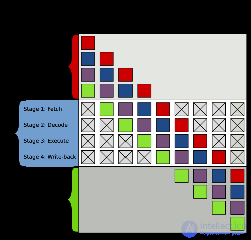
| Clock | Execution |
|---|---|
| 0 |
|
| 1 |
|
| 2 |
|
| 3 |
|
| 4 |
|
| 5 |
|
| 6 |
|
| 7 |
|
| 8 |
|
| 9 |
|
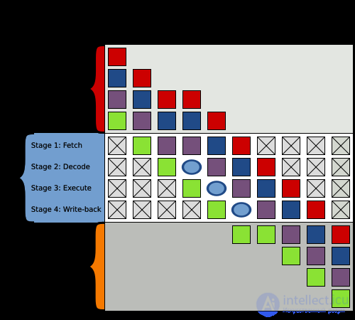
A pipelined processor can handle hazards by stalling and creating a “bubble” in the pipeline, resulting in one or more cycles in which nothing useful happens.
In the illustration on the right, in cycle 3 the processor cannot decode the purple instruction, possibly because it determines that decoding depends on results produced by the execution of the green instruction. The green instruction can proceed to the execute stage and then to the write-back stage as scheduled, but the purple instruction is delayed by one cycle at the fetch stage. The blue instruction, which should have been fetched during cycle 3, is delayed by one cycle, as is the red instruction that follows it.
Because of the bubble (the blue ovals in the illustration), the decode circuitry of the processor is idle during the 3rd cycle. The execute circuitry is idle during the 4th cycle, and the write-back circuitry is idle during the 5th cycle.
When the bubble exits the pipeline (in the 6th cycle), normal execution resumes. But now everything is one cycle behind. Fully executing the four instructions shown in color will take 8 cycles (from the 1st through the 8th). [ b ]

Comments