The Viterbi Algorithm

The Viterbi algorithm is an algorithm for finding the most suitable list of states (called the Viterbi path) that, in the context of Markov chains, yields the most probable sequence of events that occurred.

It is a dynamic programming algorithm. It is used in the Viterbi convolutional decoding algorithm.

The algorithm was proposed by Andrew Viterbi in 1967 as a decoding algorithm for convolutional codes transmitted over noisy networks. The algorithm found wide application in decoding the convolutional codes of GSM and CDMA mobile phones, dial-up modems and 802.11 wireless networks. It is also widely used in speech recognition, speech synthesis, computational linguistics and bioinformatics. For example, in speech recognition the audio signal is treated as a sequence of observed events, and the text string is the "hidden meaning" of the acoustic signal. The Viterbi algorithm finds the most probable text string for a given signal.

The algorithm makes several assumptions:

• the observed and hidden events must be a sequence. The sequence is most often ordered by time.
• the two sequences must be aligned: each observed event must correspond to exactly one hidden event
• computing the most probable hidden sequence up to time t must depend only on the observed event at time t and on the most probable sequence up to time t − 1.

Algorithm

Suppose there is a hidden Markov model (HMM) with a state space , where is the number of possible distinct states of the network. The states the network takes on are not visible to observation. Denote by the state of the network at time . At the network output at time an observable value appears, where is the number of possible distinct observable output values. Let be the initial probability of the network being in the state the probabilities of transition of the network from the state to the state .

Let the sequence be observed at the network output. Then the most probable sequence of network states for the observed sequence can be determined using the following recurrence relations

Here is the probability of the most probable state sequence corresponding to the first observed values, ending in the state . The Viterbi path can be found using pointers that remember which state occurred in the second equation. Let be a function that returns the value used to compute if , or if . Then

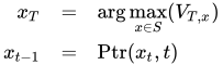
Here we use the standard definition of arg max.
The complexity of this algorithm is .

Extensions

A generalization of the Viterbi algorithm, called the max-sum algorithm (or max-product algorithm ), can be used to find the most probable assignment of all or some subset of the hidden variables in a large number of graphical models , for example Bayesian networks , Markov random fields and conditional random fields . The hidden variables generally must be connected in a manner somewhat similar to a hidden Markov model (HMM), with a limited number of connections between variables and some type of linear structure among the variables. The general algorithm involves message passing and is essentially similar to the belief propagation algorithm (which is a generalization of the forward-backward algorithm ).

Using an algorithm called iterative Viterbi decoding, one can find the subsequence of an observation that best (on average) matches a given hidden Markov model. This algorithm was proposed by Qi Wang et al. to deal with turbo codes . Iterative Viterbi decoding works by iteratively invoking a modified Viterbi algorithm, re-estimating the score for a filler until convergence.

An alternative algorithm, the lazy Viterbi algorithm, has been proposed. For many applications of practical interest, under reasonable noise conditions the lazy decoder (using the lazy Viterbi algorithm) is much faster than the original Viterbi decoder (using the Viterbi algorithm). While the original Viterbi algorithm computes every node in the trellis of possible outcomes, the lazy Viterbi algorithm maintains a priority list of nodes to evaluate in order, and the number of computations required is generally smaller (and never greater) than for the ordinary Viterbi algorithm for the same result. However, it is not so easy to parallelize in hardware.

Pseudocode

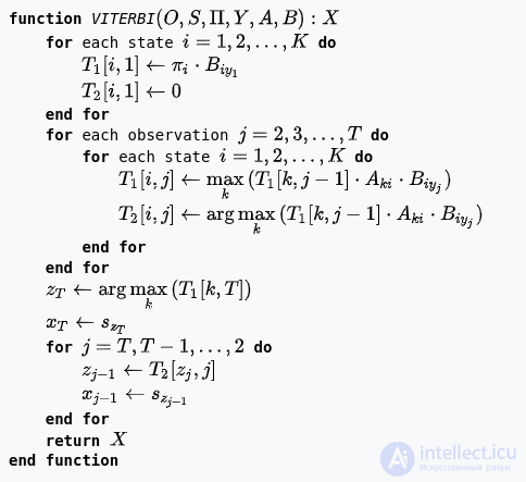
This algorithm generates a path , which is a sequence of states that generate the observations , where is the number of possible observations in the observation spaceO .

Two two-dimensional tables of sizeK×T are constructed:

• Each element of stores the probability of the most probable path so far with that generates .
• Each element ofT2 stores of the most probable path so far

The entries of the table 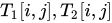are filled in order of increasing :

,

,

and as defined below. Note that does not necessarily have to appear in the last expression, since it is non-negative and does not depend on and thus does not affect the argmax.

Input

• The observation space ,
• the state space ,
• an array of initial probabilities such that stores the probability that ,
• a sequence of observations such that if the observation at time is ,
• a transition matrix A of size K×K such that stores the probability of transition from state to state ,
• an emission matrix B of size K×N such that stores the probability of observing from state .

Output

• The most likely sequence of hidden states

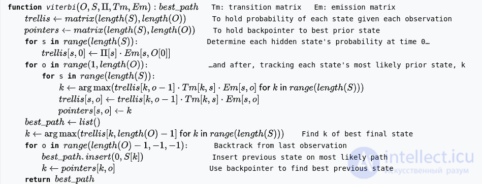
Restated in concise, Python-like form:

Explanation

Suppose we are given a hidden Markov model (HMM) with state space , initial probabilities of being in hidden stateiand transition probabilities of moving from state to state . Say we observe the outputs . The most likely state sequencex1,…,xTthat produces the observations is given by the recurrence relations

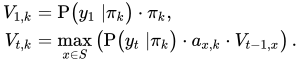
Here is the probability of the most likely state sequence responsible for the first observations that has as its final state. The Viterbi path can be obtained by saving back pointers that remember which state was used in the second equation. Let be the function that returns the value of used to compute if , or if . Then

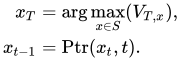
Here we use the standard definition of arg max.

The complexity of this implementation is . A better bound exists if the maximum in the inner loop is instead found by iterating only over the states that directly link to the current state (i.e. there is an edge from ). Then, using amortized analysis, one can show that the complexity is , where E is the number of edges in the graph.

Example

Consider a village where all villagers are either healthy or have a fever, and only the village doctor can determine whether each has a fever. The doctor diagnoses a fever by asking patients how they feel. The villagers can only answer that they feel normal, dizzy, or cold.

The doctor believes that the patients' health condition operates as a discrete Markov chain. There are two states, "Healthy" and "Fever", but the doctor cannot observe them directly; they are hidden from the doctor. Each day there is a certain chance that the patient will tell the doctor "I feel normal", "I feel cold", or "I feel dizzy", depending on the patient's health condition.

The observations (normal, cold, dizzy) along with the hidden state (healthy, fever) form a hidden Markov model (HMM) and can be represented as follows in the Python programming language:

obs = ("normal", "cold", "dizzy")
states = ("Healthy", "Fever")
start_p = {"Healthy": 0.6, "Fever": 0.4}
trans_p = {
    "Healthy": {"Healthy": 0.7, "Fever": 0.3},
    "Fever": {"Healthy": 0.4, "Fever": 0.6},
}
emit_p = {
    "Healthy": {"normal": 0.5, "cold": 0.4, "dizzy": 0.1},
    "Fever": {"normal": 0.1, "cold": 0.3, "dizzy": 0.6},
}

In this piece of code, start_p represents the doctor's belief about which state the HMM is in when the patient first visits (all the doctor knows is that the patient tends to be healthy). The particular probability distribution used here is not the equilibrium one, which (given the transition probabilities) is approximately {'Healthy': 0.57, 'Fever': 0.43}. transition_p represents the change of the health condition in the underlying Markov chain. In this example, a patient who is healthy today has only a 30% chance of having a fever tomorrow. emit_p represents how likely each possible observation (normal, cold, or dizzy) is, given the underlying state (healthy or fever). A healthy patient has a 50% chance of feeling normal; one who has a fever has a 60% chance of feeling dizzy.

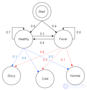
Graphical representation of the given HMM

The patient visits the doctor three days in a row, and the doctor finds that on the first day the patient feels normal, on the second day cold, and on the third day dizzy. The doctor wonders: what is the most likely sequence of the patient's health states that could explain these observations? The Viterbi algorithm answers this.

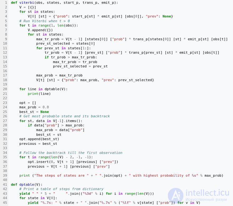
The function viterbi takes the following arguments: obs is the sequence of observations, for example ['normal', 'cold', 'dizzy']; states is the set of hidden states; start_p is the start probability; trans_p holds the transition probabilities; and emit_p holds the emission probabilities. For simplicity of the code, we assume that the observation sequence obs is non-empty and that trans_p[i] [j] and emit_p[i] [j] are defined for all states i, j.

In the working example, the forward/Viterbi algorithm is used as follows:

viterbi(obs,
        states,
        start_p,
        trans_p,
        emit_p)

Script output

$ python  viterbi_example.py
          0 1 2 
Healthy: 0.30000 0.08400 0.00588 
Fever: 0.04000 0.02700 0.01512 
State steps: Healthy Healthy Fever with highest probability 0.01512

This shows that the observations ['normal', 'cold', 'dizzy'] were most likely generated by the states ['Healthy', 'Healthy', 'Fever']. In other words, given the observed activity, the patient was most likely healthy on the first day and also on the second day (despite feeling cold that day), and only on the third day came down with a fever.

The operation of the Viterbi algorithm can be visualized with a trellis diagram. The Viterbi path is essentially the shortest path through this trellis.

See also

• [[b12028]]
• EM algorithm
• Hidden Markov model
• Expectation-maximization algorithm
• Baum–Welch algorithm
• Forward-backward algorithm
• Forward algorithm
• Error correction code
• Hidden Markov model
• Part-of-speech tagging
• A* search algorithm

See also

• Viterbi Convolutional Decoding Algorithm