
Lecture 28 min.
Transformer is a deep neural network architecture introduced in 2017 by researchers at Google Brain.
Like recurrent neural networks (RNNs), transformers are designed to process sequences, such as natural-language text, and to solve tasks such as machine translation and automatic summarization. Unlike RNNs, transformers do not require sequences to be processed in order. For example, if the input is text, the transformer does not need to process the end of the text after processing its beginning. Because of this, transformers are easier to parallelize than RNNs and can be trained faster.
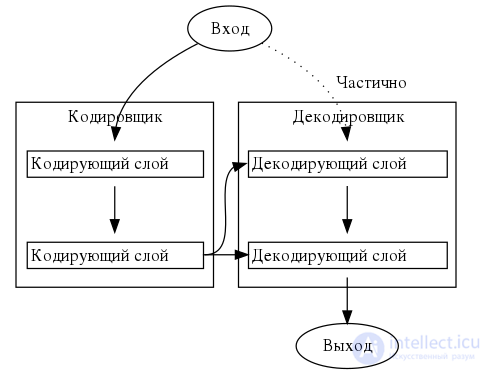
The transformer architecture consists of an encoder and a decoder. The encoder receives as input a vectorized sequence with positional information. The decoder receives as input part of this sequence and the output of the encoder. The encoder and decoder consist of layers. The encoder layers pass their result sequentially to the next layer as its input. The decoder layers pass their result sequentially to the next layer, together with the encoder's output, as its input.
Each encoder consists of a self-attention mechanism (input from the previous layer) and a feed-forward neural network (input from the self-attention mechanism). Each decoder consists of a self-attention mechanism (input from the previous layer), an attention mechanism over the encoding results (input from the self-attention mechanism and the encoder) and a feed-forward neural network (input from the attention mechanism).
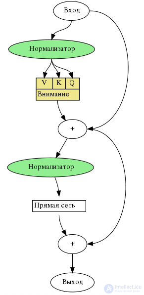
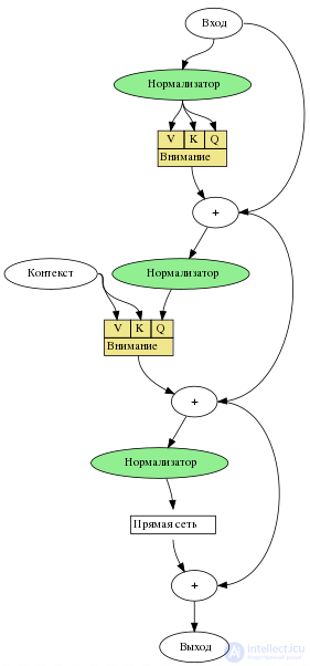
Each attention mechanism is parameterized by a query weight matrix  , a key weight matrix
 , and a value weight matrix
 . To compute the attention of an input vector 𝑋 to a vector 𝑌 , the vectors
 ,
 ,
 are computed. These vectors are used to compute the attention result by the formula:

Before transformers, predecessors of the attention mechanism, such as LSTM and gated recurrent units (GRU), were added to gated recurrent neural networks, which processed datasets sequentially. The dependence on previous token computations prevented them from parallelizing the attention mechanism. In 1992, the fast weight controller was proposed as an alternative to recurrent neural networks that can learn "internal spotlights of attention". In theory, information from one token can propagate arbitrarily far down the sequence, but in practice the vanishing gradient problem leaves the model's state at the end of a long sentence without precise, retrievable information about preceding tokens.
The performance of earlier models was improved by adding an attention mechanism, which allowed the model to access any previous point in the sequence. The attention layer weights all previous states according to a learned measure of relevance, providing relevant information about distant tokens. This proved especially useful in language translation, where distant context can be critical to the meaning of a word in a sentence. The state vector was available only after the last English word had been processed while, for example, translating it from French with an LSTM model. Although in theory such a vector retains information about the whole source sentence, in practice that information is poorly preserved. If an attention mechanism is added, the decoder is given access to the state vectors of every input word, not just the last one, and it can learn attention weights that determine how much attention to pay to each input state vector. Augmenting seq2seq models with an attention mechanism was first implemented in the context of machine translation by Bahdanau, Cho, and Bengio in 2014.
In 2016, highly parallelizable decomposable attention was successfully combined with a feedforward network. This indicated that attention mechanisms are powerful in themselves and that sequential recurrent processing of data is not necessary to achieve the quality gains of recurrent neural networks with attention. In 2017, Vaswani et al. also proposed replacing recurrent neural networks with self-attention and began efforts to evaluate this idea. Transformers, using an attention mechanism and processing all tokens simultaneously, computed "soft" weights between them in successive layers. Since the attention mechanism uses information only about other tokens from lower layers, it can be computed for all tokens in parallel, which leads to faster training.
The plain transformer architecture had difficulty converging. In the original paper the authors recommended using learning rate warmup. That is, the learning rate should increase linearly from 0 to its maximum value over the first part of training (usually recommended to be 2% of the total number of training steps), and then decrease again.
A 2020 paper found that applying layer normalization before (rather than after) the multi-head attention and feedforward layers stabilizes training, without requiring learning rate warmup.
The GT 3 model combines CWTE, SWTE, and TTE using a self-adaptive gate layer, which enables an efficient and effective fusion of the three types of features for end-to-end text-based stock market prediction.
Transformers typically undergo self-supervised learning, involving unsupervised pretraining followed by supervised fine-tuning. Pretraining is usually done on a larger dataset than fine-tuning, due to the limited availability of labeled training data. Pretraining and fine-tuning tasks commonly include:
The paper on the T5 transformer documents a large number of pretraining tasks. Some examples are:
Thank you <X> me to your party <Y> week.-> <X> for inviting <Y> last <Z>where <Z>means "end of output".translate English to German: That is good.-> Das ist gut..The course is jumping well. ): -> not acceptable.The transformer model is implemented in standard deep learning frameworks such as TensorFlow and PyTorch .
Transformers is a library created by Hugging Face , which provides transformer-based architectures and pretrained models.
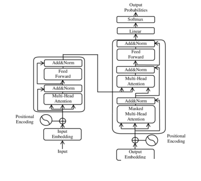
An illustration of the main components of the transformer model from the original paper, where layer normalization was applied after multi-head attention. A 2020 paper found that placing layer normalization before multi-head attention (rather than after it) improves training stability .
All transformers have the same primary components:
Transformer layers can be one of two types: encoder and decoder . The original paper used both, whereas later models included only one of them. BERT is an example of an encoder-only model; GPT models are decoder-only.
The input text is parsed into tokens by a tokenizer, most often a byte-pair encoding tokenizer , and each token is converted into a vector by looking it up in a word embedding table . Then the positional information of the token is added to the word embedding.
Like earlier seq2seq models , the original transformer model used an encoder-decoder architecture . The encoder consists of encoding layers that iteratively process the input tokens one layer after another, while the decoder consists of decoding layers that iteratively process the encoder's output as well as the decoder's output tokens.
The function of each encoder layer is to generate contextualized token representations, where each representation corresponds to a token that "mixes" information from the other input tokens via the self-attention mechanism. Each decoder layer contains two attention sublayers: (1) cross-attention for incorporating the encoder output (contextualized input token representations) and (2) self-attention for "mixing" information among the input tokens to the decoder (i.e. the tokens generated so far during inference)
Both the encoder and decoder layers have a feedforward neural network for additional processing of the outputs, and contain residual connections and layer normalization steps.
The building blocks of the transformer are scaled dot-product attention units . For each attention unit, the transformer model learns three weight matrices: the query weights , the key weights , and the value weights . For each token  , the input token representationxi
 is multiplied by each of the three weight matrices to produce a query vector q
 , a key vectorki=xiWK
 , and a value vector v
 . The attention weights are calculated using the query and key vectors: the attention weight
 from token to token
 is the dot product betweenqi
 andkj
 . The attention weights are divided by the square root of the dimension of the key vectors,dk
 , which stabilizes gradients during training, and passed through a softmax , which normalizes the weights. The fact that and are different matrices allows attention to be non-symmetric: if tokeniattends to tokenj(i.e.
 is large), this does not necessarily mean that token will attend to tokeni(i.e.
 may be small). The output of the attention unit for tokeniis the weighted sum of the value vectors of all tokens, weighted by , the attention from token to each token.
The attention calculation for all tokens can be expressed as one large matrix calculation using the softmax function , which is useful for training because of computational matrix operation optimizations that allow matrix operations to be computed quickly. The matrices  ,
 and
 are defined as the matrices whoseith rows are the vectors ,
 , and
 respectively. Then we can represent the attention as

where the softmax is taken over the horizontal axis.
One set of  matrices is called an attention head , and each layer in a transformer model has multiple attention heads. While each attention head attends to the tokens that are relevant to each token, multiple attention heads allow the model to do this for different definitions of "relevance". In addition, the field of influence representing relevance can become progressively dilated in successive layers. Many transformer attention heads encode relevance relations that are meaningful to humans. For example, some attention heads may attend mostly to the next word, while others mainly attend from verbs to their direct objects. The computations for each attention head can be performed in parallel , which allows for fast processing. The outputs of the attention layer are concatenated to be passed into the feedforward neural network layers .
Concretely, let the multiple attention heads be indexed byi, then we have

where the matrix  is the concatenation of word embeddings, and the matrices
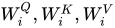 are the "projection matrices" belonging to an individual attention head , and
 is a final projection matrix belonging to the whole multi-head attention head.
It may be necessary to cut out attention links between some pairs of words. For example, the decoder at token positiont should not have access to token position
 . This can be done before the softmax stage by adding a mask matrixM that is
 at entries where the attention link must be disabled, and0 elsewhere:

For example, autoregressive modeling uses the following mask matrix:
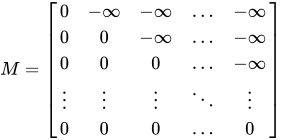
In words, this means that each token can attend to itself and every token before it, but not to any token after it.
Each encoder consists of two major components: a self-attention mechanism and a feedforward neural network. The self-attention mechanism accepts input encodings from the previous encoder and weighs their relevance to each other to generate output encodings. The feedforward neural network further processes each output encoding individually. These output encodings are then passed to the next encoder as its input, as well as to the decoders.
The first encoder takes positional information and embeddings of the input sequence as its input, rather than encodings. The positional information is necessary for the transformer to make use of the order of the sequence, because no other part of the transformer makes use of it.
The encoder is bidirectional. Attention can be paid to tokens both before and after the current token. Tokens are used instead of words to account for polysemy .
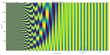
Diagram of sinusoidal positional encoding with parameters 
Positional encoding is a fixed-size vector representation that encapsulates the relative positions of tokens within a target sequence: it provides the transformer model with information about where the words are in the input sequence.
Positional encoding is defined as a function of type  , where
 is a positive even integer . The full positional encoding defined in the original paper is given by the equation:

where 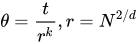 .
Here,  is a free parameter that should be significantly larger than the biggest
 that would be input into the positional encoding function. In the original paper the authors chose
 .
The function has a simpler form when written as a complex function of typef: 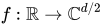
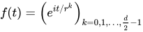
where  .
The main reason the authors chose this as the positional encoding function is that it allows shifts to be performed as linear transformations:

where  is the distance one wishes to shift. This allows the transformer to take any encoded position and find the encoding of the position n steps ahead or n steps behind, by a matrix multiplication.
By taking a linear sum, any convolution can also be implemented as linear transformations:

for any constantscj . This allows the transformer to take any encoded position and find a linear sum of the encoded locations of its neighbors. This sum of encoded positions, when fed into the attention mechanism, would create attention weights on its neighbors, much like what happens in a convolutional neural network language model . In the authors' words, "we hypothesized it would allow the model to easily learn to attend by relative position."
In typical implementations, all operations are done over the real numbers, not the complex numbers, but since complex multiplication can be implemented as real 2-by-2 matrix multiplication , this is just a difference in notation.
Each decoder consists of three major components: a self-attention mechanism, an attention mechanism over the encodings, and a feedforward neural network. The decoder functions in a similar way to the encoder, but an additional attention mechanism is inserted which instead draws relevant information from the encodings generated by the encoders. This mechanism can also be called encoder-decoder attention .
Like the first encoder, the first decoder takes positional information and embeddings of the output sequence as its input, rather than encodings. The transformer must not use the current or future output to predict an output, so the output sequence must be partially masked to prevent this reverse information flow. This allows for autoregressive text generation. For all attention heads, attention cannot be paid to following tokens. The last decoder is followed by a final linear transformation and softmax layer, to produce the output probabilities over the vocabulary.
All members of the OpenAI GPT series have a decoder-only architecture.
In large language models, the terminology is somewhat different from that used in the original Transformer paper:
Here "autoregressive" means that a mask is inserted in the attention head to zero out all attention from one token to all tokens following it, as described in the "Masked attention" section.
Generally, transformer-based language models are of two types: causal (or "autoregressive") and masked. The GPT series is causal and decoder-only. BERT is masked and encoder-only. The T5 series is encoder-decoder, with a full encoder and an autoregressive decoder.
The original transformer uses the ReLU activation function. Other activation functions have been developed, such as SwiGLU
Transformers may use positional encoding methods other than sinusoidal.
RoPE (rotary positional embedding) is best explained by considering a list of 2-dimensional vectors  . Now pick an angleθ
 . Then the RoPE encoding is

Equivalently, if we write the 2-dimensional vectors as complex numberszm=xm(1)+ixm(2) , then the RoPE encoding is just multiplication by an angle:

For a list of  -dimensional vectors, a RoPE encoder is defined by a sequence of angles
 . Then the RoPE encoding is applied to each pair of coordinates.
The advantage of RoPE is that the dot product between two vectors depends only on their relative location:

for any integer .
ALiBi (Attention with Linear Biases) is not a replacement for the positional encoder of the original transformer. Instead, it is an additional positional encoder that is directly plugged into the attention mechanism. Specifically, the ALiBi attention mechanism is

Here,s is a real number (a "scalar"), and
 is the linear bias matrix, defined by
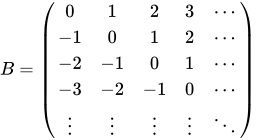
in other words,  .
ALiBi allows pretraining on short context windows, then fine-tuning on longer context windows. Since it is directly plugged into the attention mechanism, it can be combined with any positional encoder that is plugged into the "bottom" of the entire network (which is where the sinusoidal encoder on the original transformer, as well as RoPE and many others, are located).
Relative positional encoding is similar to ALiBi, but more generic:

where is a Toeplitz matrix , that is,  wheneveri−
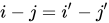 .
FlashAttention is an algorithm that implements the transformer attention mechanism efficiently on a GPU. It performs matrix multiplications in blocks , such that each block fits within the GPU cache, and by careful management of the blocks it minimizes data copying between GPU caches (as data movement is slow).
An improved version, FlashAttention-2, was developed to meet the growing demand for language models capable of processing longer contexts. It offers improvements in work partitioning and parallelism, enabling it to achieve up to 230 TFLOPs/s on A100 GPUs ( FP16 / BF16 ), a 2x speedup over the original FlashAttention.
Key advances in FlashAttention-2 include reducing the number of non-matmul FLOPs, improved parallelism over the sequence length dimension, better work partitioning between GPU warps, and added support for head sizes up to 256 as well as multi-query attention (MQA) and grouped-query attention (GQA).
Benchmarks revealed that FlashAttention-2 is up to 2x faster than FlashAttention and up to 9x faster than a standard attention implementation in PyTorch. Future developments include optimization for new hardware such as H100 GPUs and new data types such as FP8.
Multi-query attention changes the multi-head attention mechanism. Whereas normally,
with multi-query attention there is just oneWK,WV , thus:

This has a neutral effect on model quality and training speed, but increases inference speed.
Transformers are used in large language models for autoregressive sequence generation: generating a stream of text, one token at a time. However, in most settings, decoding from language models is memory-bound, meaning that we have spare compute power available. Speculative decoding [ uses this spare compute power by computing several tokens in parallel. Similarly to speculative execution in CPUs, future tokens are computed concurrently, by speculating on the value of previous tokens, and are then discarded if it turns out the speculation was incorrect.
In particular, consider a transformer model like GPT-3, which has a context window size of 512. To generate an entire context window autoregressively with greedy decoding, it would have to be run 512 times, generating one token each time.  . However, if we had some educated guess for the values of these tokens, we could verify all of them in parallel, in one run of the model, by checking that each
 is indeed the token with the largest log-likelihood in the -th output.
In speculative decoding, a smaller model or some other simple heuristic is used to generate a few speculative tokens that are subsequently verified by the larger model. For example, suppose a small model generated four speculative tokens:  . These tokens are run through the larger model, and only
 and
 are accepted. The same run of the large model has already generated a new token
 to replace
 , andx4~
 is completely discarded. The process then repeats (starting from the 4th token) until all tokens are generated.
For non-greedy decoding, similar ideas apply, except that the speculative tokens are accepted or rejected stochastically, in such a way as to guarantee that the final output distribution is the same as if speculative decoding were not used.
Training transformer-based architectures can be expensive, especially for long inputs. Alternative architectures include the Reformer (which reduces the computational load from  to
 ) or models like ETC/BigBird (which can reduce it to
 ) where is the length of the sequence. This is done using locality-sensitive hashing and reversible layers.
Ordinary transformers require a memory size that is quadratic in the size of the context window. Attention-free transformers reduce this dependence to linear while still retaining the advantages of the transformer by linking the key to the value.
Long Range Arena (2020) is a standard benchmark for comparing the behavior of transformer architectures over long inputs.
Random Feature Attention (2021) uses random Fourier features:

where  are independent samples from the normal distribution
 . This choice of parameters satisfies
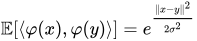 , or

Consequently, the unidirectional attention with a single query can be written as

where  . Similarly for multiple queries and multi-headed attention.
This approximation can be computed in linear time, since we can compute the matrix  first, then multiply it by the query. Essentially, we have managed to obtain a more precise version of

Performer (2022) uses the same random feature attention, but are first independently sampled from the normal distribution , and then they are processed with Gram-Schmidt.
Transformers can also be used or adapted for modalities (input or output) beyond text, usually by finding a way to "tokenize" the modality.
Vision transformers adapt the transformer to computer vision by breaking input images into a series of patches, turning them into vectors, and treating them as tokens in a standard transformer.
Conformer and the later Whisper follow the same pattern for speech recognition , first turning the speech signal into a spectrogram , which is then treated like an image, i.e., broken into a series of patches, turned into vectors, and treated as tokens in a standard transformer.
Perceivers , by Andrew Jaegle et al. (2021) can learn from large amounts of heterogeneous data.
As for image output , Peebles et al. introduced the Diffusion Transformer (DiT), which facilitates the use of the transformer architecture for diffusion-based image generation . In addition, Google released a transformer-centric image generator called "Muse", based on parallel decoding and the masked generative transformer technique. (Transformers played a less central, though still significant, role in earlier image generation technologies. )
The transformer has had great success in natural language processing (NLP), for example in machine translation and time series prediction tasks. Many large language models , such as GPT-2 , GPT-3 , GPT-4 , Claude , BERT , XLNet, RoBERTa and ChatGPT, demonstrate the ability of transformers to perform a wide variety of such NLP-related tasks, and have the potential to find real-world applications. These may include:
Beyond NLP applications, it has also had success in other areas, such as computer vision or protein folding applications (such as AlphaFold ).
As an illustrative example, consider Ithaca, an encoder-only transformer with three output heads. It takes an ancient Greek inscription as input in the form of a sequence of characters, but with illegible characters replaced by "-". Its three output heads respectively output probability distributions over Greek characters, the location of the inscription, and the date of the inscription.
Sign in and the lectures you have studied will be marked in this list.
Choose a course
Comments