Lecture
Perceptron , or pen with epptron (English perceptron from the Latin. Perceptio - perception; German. Perzeptron ) - a mathematical or computer model of information perception by the brain (cybernetic model of the brain ), proposed by Frank Rosenblatt in 1957 and implemented as an electronic machine "Mark-1" in 1960. Perceptron was one of the first models of neural networks , and Mark-1 - the world's first neurocomputer . Despite its simplicity, the perceptron is capable of learning and solving fairly complex tasks. The main mathematical problem with which he copes is the linear separation of any non-linear sets, the so-called ensuring linear separability.
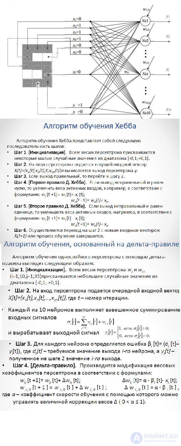
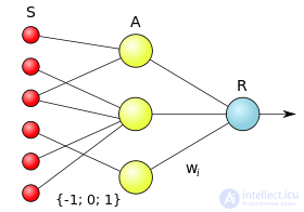
A perceptron consists of three types of elements, namely: signals coming from sensors are transmitted to associative elements, and then reacting elements. Thus, perceptrons allow you to create a set of "associations" between input stimuli and the necessary response at the output. In biological terms, this corresponds to the transformation, for example, of visual information into a physiological response from motor neurons. According to modern terminology, perceptrons can be classified as artificial neural networks:
Against the background of the growing popularity of neural networks in 1969, the book by Marvin Minsky and Seymour Papert was published, which showed the fundamental limitations of perceptrons. This led to a shift in the interest of researchers of artificial intelligence in the field of symbolic calculations opposite to neural networks. . In addition, due to the complexity of the mathematical analysis of perceptrons, as well as the lack of generally accepted terminology, various inaccuracies and delusions have arisen.
Subsequently, interest in neural networks, and in particular, the work of Rosenblatt, resumed. So, for example, biocomputing is developing rapidly, which, in its theoretical basis of computation, is based on neural networks, and reproduces the perceptron based on bacteriorhodopsin-containing films.

There are two classes of tasks solved by the trained neural networks. These are the tasks of prediction and classification.
The tasks of prediction or forecasting are, in essence, the tasks of constructing a regression dependence of the output data on the input data. Neural networks can effectively build highly non-linear regression dependencies. The specificity here is such that, since mostly non-formalized tasks are solved, the user is primarily interested not in building a clear and theoretically justified relationship, but in obtaining a predictor device. The forecast of such a device will not directly go into action - the user will evaluate the output signal of the neural network based on his knowledge and form his own expert opinion. The exceptions are situations, based on the trained neural network create a control device for the technical system.
When solving classification problems, a neural network builds a dividing surface in the attribute space, and the decision on whether a particular class belongs to a particular class is made by an independent, network-independent device — the interpreter of the network response. The simplest interpreter arises in the problem of binary classification (classification into two classes). In this case, one output signal of the network is sufficient, and the interpreter, for example, relates the situation to the first class if the output signal is less than zero and to the second if it is greater than or equal to zero.

Structure and properties of an artificial neuron
The neuron is an integral part of the neural network. In fig. 2 shows its structure. It consists of three types of elements: multipliers (synapses), adder and non-linear transducer. Synapses communicate between neurons, multiply the input signal by a number characterizing the strength of the connection, (the weight of the synapse). The adder performs the addition of signals coming in via synaptic connections from other neurons and external input signals. Nonlinear converter implements a nonlinear function of one argument - the output of the adder. This function is called the activation function or transfer function of the neuron.
Fig. 2. Structure of an artificial neuron
The neuron as a whole implements the scalar function of the vector argument. Mathematical model of neuron:
|
|
(1.1) |
|
|
y = f (s) |
|
(1.2) |
where wi, is the weight (weight) of the synapse, i = 1 ... n; b is the bias value (bias); s is the result of summation (sum); x, is the component of the input vector (input signal), xi = 1 ... n; y is the output of the neuron; n is the number of inputs of the neuron; f is a non-linear transformation (activation function).
In the general case, the input signal, the weighting factors and the offset can take real values, and in many practical problems only some fixed values. Output (y) is determined by the type of activation function and can be both real and whole.
Synaptic connections with positive weights are called excitatory , with negative weights inhibitory .
The described computational element can be considered a simplified mathematical model of biological neurons. To emphasize the difference between biological and artificial neurons, the latter are sometimes called neuron-like elements or formal neurons.
The nonlinear converter responds to the input signal (s) with the output signal f (s), which is the output from the neuron. Examples of activation functions are presented in Table. 1. and fig. 3
Table 1
Fig. 3. Examples of activation functions
a is the single jump function; b - linear threshold (hysteresis);
в - sigmoid (logistic function); d - sigmoid (hyperbolic tangent)Table 2. The main options for describing the activation function
One of the most common is the nonlinear activation function with saturation, the so-called logistic function or sigmoid (S-shaped function):
|
f (s) = 1 / (1 + e -as) |
(1.3) |
As a decreases, the sigmoid becomes flatter, in the limit at a = 0, degenerating into a horizontal line at 0.5, with increasing a, the sigmoid approaches the form of the single hop function with a threshold of 0. From the expression for the sigmoid it is obvious that the output value of the neuron range (0, 1). One of the valuable properties of the sigmoidal function is a simple expression for its derivative, the application of which will be considered further:
|
f '(s) = af (s) [1 -f (s)] |
(1.4) |
It should be noted that the sigmoidal function is differentiable on the entire abscissa axis, which is used in some learning algorithms. In addition, it has the ability to amplify weak signals better than large ones and prevents saturation from large signals, since they correspond to areas of arguments where the sigmoid has a gentle slope.
Model of a formal cybernetic neuron.
A formal neuron consists of 3 logical blocks: inputs, transformation function, output. Let us consider in more detail the conversion function block.
Figure 4. Model of a formal neuron. The dashed box marks the transform function block.
As a conversion function, the following are commonly used:
- simple threshold
- Lenin-threshold function
- sigmoid
Examples of the simplest tasks
1. Calculate the network output of a perceptron with a bipolar sigmoidal activation function,
if the following parameters are known: x1 = 0.7; w1 = 1.5; x2 = 2.5; w2 = -1; b = 0.5.
2. Calculate the network output of the perceptron with the unipolar sigmoidal activation function,
if the following parameters are known: x1 = 0.7; w1 = 1.5; x2 = 2.5; w2 = -1; b = 0.5.
The solution of the simplest abstract problem
activation function: y = f (s)
The value of the activation function is calculated by the formula
k - accept any number
Comments
To leave a comment
Neural networks
Terms: Neural networks