
Lecture
In machine learning, attention is a technique that determines the importance of each component in a sequence relative to the other components in that sequence. In natural language processing, importance is represented by “soft” weights assigned to each word in a sentence. More generally, attention encodes vectors called token embeddings into a sequence of fixed width, whose size can range from tens to millions of tokens.
Unlike “hard” weights, which are computed during the backward pass of training, “soft” weights exist only in the forward pass and therefore change at every step of the input data. In earlier designs, attention was implemented in a language-translation system based on a sequential recurrent neural network (RNN), but in a later design, namely the Transformer, the slower sequential RNN was removed and a faster, parallel attention scheme was relied on instead.
Inspired by ideas about attention in humans, attention was designed to address the shortcomings of using information from the hidden layers of recurrent neural networks. Recurrent neural networks favor more recent information contained in words toward the end of a sentence, while information located near the beginning of the sentence tends to be less significant. Attention allows a token to gain equal access to any part of the sentence directly, rather than only through the previous state.
| 1950s – 1960s | Psychology and biology of attention. The “cocktail party” effect — focusing on content by filtering out background noise. Filter models of attention, the partial report paradigm, and control of saccades. |
| 1980s | Sigma-pi units, higher-order neural networks. |
| 1990s | Fast weight controllers and dynamic connections between neurons, anticipating key-value mechanisms in attention. |
| 1998 | The bilateral filter was introduced in image processing. It uses pairwise similarity matrices to propagate relevance between elements. |
| 2005 | Non-local means extended similarity-based filtering in image denoising, using Gaussian similarity kernels as fixed weights analogous to attention. |
| 2014 | seq2seq with RNN + Attention. Attention was introduced to improve RNN encoder-decoder translation, especially for long sentences. See the “Overview” section.
Attention neural networks introduced a learned feature-selection mechanism using top-down cognitive modulation, demonstrating how attention weights can highlight relevant input. |
| 2015 | Attention was extended to vision for image-captioning tasks. |
| 2016 | A self-attention mechanism was integrated into an RNN-based model to account for intra-sequence dependencies.
Self-attention was explored in decomposable attention models for natural language inference and in structured self-attentive sentence embeddings. |
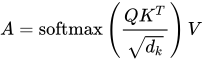
| 2017 | The Transformer architecture, introduced in the research paper Attention Is All You Need, formalized scaled dot-product self-attention:
Relation networks and set transformers apply attention to unordered sets and relational reasoning, generalizing pairwise-interaction models. |
| 2018 | Non-local neural networks extended the capabilities of computer vision by capturing long-range dependencies in space and time. Graph attention networks applied attention mechanisms to data with a graph structure. |
| 2019–2020 | Efficient transformers, including Reformer , Linformer and Performer , introduced scalable approximations of attention for long sequences. |
| 2019+ | Hopfield networks were reinterpreted as memory-based associative attention systems , while vision transformers (ViT) achieved competitive results in image classification .
Transformers have been applied in various scientific fields, including AlphaFold for protein folding , CLIP for image-language pretraining and attention-based dense segmentation models such as CCNet and DANet . |
Further research on attention mechanisms in deep learning is presented in the work of Niu et al. and Soydaner.
The major breakthrough came from the self-attention mechanism, in which every element of the input sequence attends to all the others, allowing the model to capture global dependencies. This idea was central to the Transformer architecture, which replaced recurrence with attention mechanisms. As a result, Transformers became the foundation for models such as BERT, T5, and generative pre-trained transformers (GPT).
The modern era of machine attention gained new momentum from the introduction of an attention mechanism (fig. 1, orange) into the encoder-decoder.
|
|
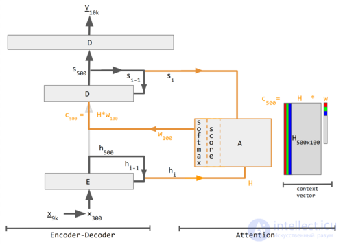 Fig. 1. Encoder-decoder with attention mechanism. The numeric indices (100, 300, 500, 9k, 10k) indicate vector sizes, and the letter indices i and i − 1 indicate time steps. The pink regions in matrix H and vector w are zero values. See the legend for details. Fig. 1. Encoder-decoder with attention mechanism. The numeric indices (100, 300, 500, 9k, 10k) indicate vector sizes, and the letter indices i and i − 1 indicate time steps. The pink regions in matrix H and vector w are zero values. See the legend for details. |
| Symbol | Description |
|---|---|
| 100 | Maximum sentence length |
| 300 | Embedding size (word dimensionality) |
| 500 | Length of hidden vector |
| 9k, 10k | Vocabulary size for the input and output languages respectively. |
| x, Y | 9k and 10k 1-hot vocabulary vectors. x → x is implemented as a lookup table, rather than as a vector multiplication. Y is the 1-hot maximizer of the decoder D's linear layer; that is, it takes the argmax of the output of linear layer D. |
| x | Word embedding vector of length 300. The vectors are usually precomputed from data of other projects, such as GloVe or Word2Vec. |
| h | Encoder hidden vector of length 500 characters. At each point in time, this vector sums up all the words preceding it. The final h can be regarded as a “sentence” vector, or, as Hinton calls it, a thought vector. |
| s | Decoder hidden state vector of length 500. |
| E | Encoder based on a recurrent neural network with 500 neurons . 500 outputs. Number of inputs: 800 – 300 from the source embedding + 500 from the recurrent connections. The encoder feeds the decoder directly only to initialize it, but not afterward; hence this direct connection is drawn very faintly. |
| D | 2-layer decoder. The recurrent layer has 500 neurons, and the fully connected linear layer has 10,000 neurons (target vocabulary size). Only the linear layer has 5 million (500 × 10,000) weights — roughly 10 times as many weights as the recurrent layer. |
| score | 100-value alignment score |
| w | Attention vector weights of length 100. These are “soft” weights, which change during the forward pass, unlike “hard” neural weights, which change during the training phase. |
| A | Attention module – this can be a dot product of recurrent states or fully connected “query-key-value” layers. The output is a vector of length 100, w. |
| H | 500×100. 100 hidden vectors h combined into a matrix. |
| c | Context vector of length 500 = H * w. c is a linear combination of the h vectors, weighted by w. |
Figure 2 shows the internal, step-by-step operation of the attention block (A) in figure 1.
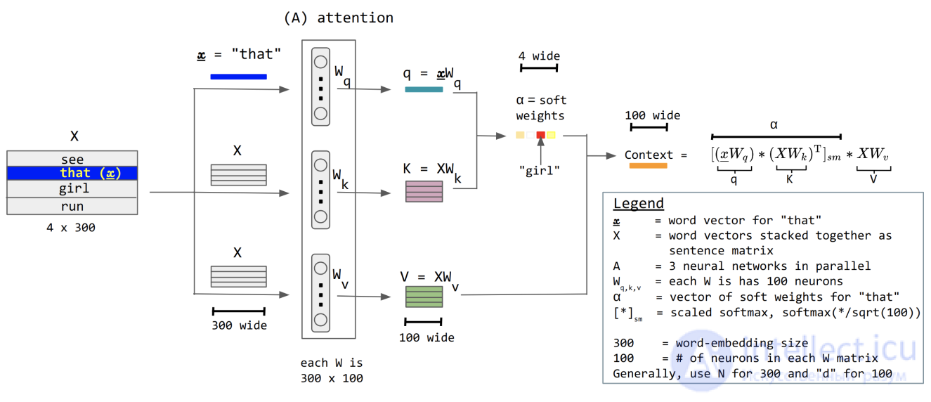
Figure 2. The diagram shows how the attention algorithm computes the correlations of the word “that” with the other words in the phrase “See that girl run”. With a proper distribution of the weights learned during training, the network should be able to identify the word “girl” as the highly correlated word. Some important points:
 .
.
When translating between languages, alignment is the process of mapping words in the source sentence to words in the translated sentence. Neural networks that perform word-for-word translation without regard to word order show the highest scores along the (dominant) diagonal of the matrix. Dominance off the diagonal indicates a more subtle attention mechanism.
Consider the example of translating the phrase “I love you” into French. On the decoder's first pass, 94% of attention falls on the first English word “I”, so the network proposes the word “je”. On the decoder's second pass, 88% of attention falls on the third English word “you”, so the word “t'” is proposed. On the last pass, 95% of attention falls on the second English word “love”, so the word “aime” is proposed.
In the example “I love you”, the second word “love” is aligned with the third word “aime”. Stacking the soft weight vector rows for the words “je”, “t'”, and “aime” gives an alignment matrix:
| I | love | you | |
|---|---|---|---|
| je | 0.94 | 0.02 | 0.04 |
| t' | 0.11 | 0.01 | 0.88 |
| aime | 0.03 | 0.95 | 0.02 |
Sometimes alignment can be many-to-many. For example, the English phrase look it up corresponds to cherchez-le. Thus, “soft” attention weights work better than “hard” attention weights (setting one attention weight to 1 and the rest to 0), because we want the model to produce a context vector consisting of a weighted sum of hidden vectors, rather than the “single best” one, since the single best hidden vector may not exist.
Many variants of the attention mechanism use soft weights, for example:
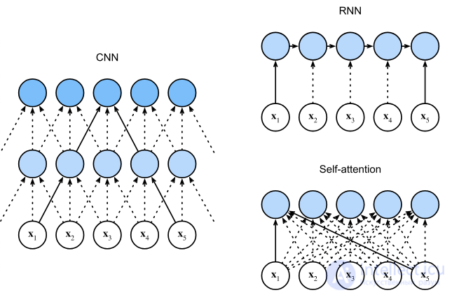
Comparison of data flow in CNN, RNN, and the self-attention mechanism
For convolutional neural networks, attention mechanisms can be distinguished by the dimension along which they operate, namely: spatial attention, channel attention, or a combination of both.
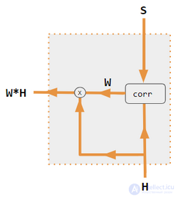
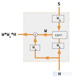
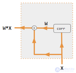
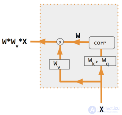
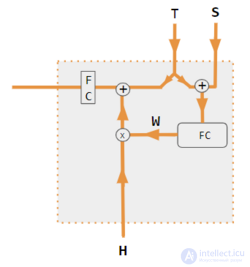
These variants recombine input data on the encoder side to redistribute these effects to each target output. Often the reweighting coefficients form a matrix of dot products in a correlation style. In the figures below, W is the context attention weight matrix, analogous to the formula in the “Overview” section above.
| 1. encoder-decoder dot product | 2. encoder-decoder QKV | 3. encoder-only dot product | 4. encoder-only QKV | 5. PyTorch tutorial |
|---|---|---|---|---|
|
|
|
|
|
The size of the attention matrix is proportional to the square of the number of input tokens. Therefore, when the input is long, computing the attention matrix requires a large amount of GPU memory. Flash attention is an implementation that reduces the memory requirement and improves efficiency without sacrificing accuracy. It achieves this by splitting the attention computation into smaller blocks that fit into the GPU's faster on-chip memory, reducing the need to store large intermediate matrices and thereby lowering memory usage while increasing computational efficiency.
FlexAttention is an attention kernel developed by Meta that allows users to modify attention scores before the softmax and dynamically select the optimal attention algorithm.
The attention mechanism is widely used in natural language processing, computer vision, and speech recognition. In NLP, it improves contextual understanding in tasks such as question answering and summarization. In computer vision, visual attention helps models focus on relevant regions of an image, improving object detection and image captioning.
Beginning with the original paper on vision transformers (ViT), visualizing attention scores as a heat map (known as saliency maps or attention maps) has become an important and standard way to analyze the decision-making process of ViT models. Attention maps can be computed with respect to any attention element at any layer, with deeper layers generally showing more semantically meaningful visualizations. The Attention Rollout algorithm is a recursive algorithm for combining attention scores across all layers by computing the dot product of successive attention maps.
Because vision transformers are typically trained in a self-supervised regime, attention maps tend not to be class-sensitive. When a classification head is attached to the base ViT network, class-discriminative attention maps (CDAM) combine attention maps with gradients with respect to the [CLS] class token. Some class-sensitive interpretability methods originally developed for convolutional neural networks can also be applied to ViT, such as GradCAM, which backpropagates gradients to the outputs of the final attention layer.
Using attention as a basis for explaining transformers in language and vision is not without controversy. While some pioneering work has analyzed and framed attention scores as explanations, higher attention scores do not always correlate with greater influence on model performance.
For matrices: and
and the scaled dot product, or QKV attention mechanism, is defined as follows:
 where
where denotes transpose, and the softmax function is applied independently to each row of its argument.
 contains
 queries, and the matrices
 jointly contain an unordered set of
 key-value pairs. The value vectors in the matrix
 are weighted using the weights obtained from the softmax operation, so that the rows -by-
 of the output matrix are confined to the convex hull of the points in
 given by the rows of.
To understand the permutation invariance and equivariance properties of QKV attention, ] let and
and be permutation matrices; and
 an arbitrary matrix. The softmax function is permutation-equivariant in the sense that:
 Given that the transpose of a permutation matrix is also its inverse, it follows that:
 which shows that the QKV attention mechanism is equivariant with respect to reordering the queries (the rows ofand invariant to reordering the key-value pairs inThese properties are inherited when linear transformations are applied to the inputs and outputs of QKV attention blocks. For example, a simple self-attention function is defined as follows:
 is permutation-equivariant with respect to permuting the rows of the input matrix
 in a nontrivial way, since each row of the output is a function of all rows of the input. Similar properties hold for multi-head attention, which is defined below.
When the QKV attention mechanism is used as a building block for an autoregressive decoder, and when during training all the input and output matrices have rows, a masked-attention variant is used: where the mask,
 is a strictly upper triangular matrix, having zeros on and below the diagonal.
 in every element above the diagonal. The output of the softmax function, likewise in
 in this case yields a lower triangular structure with zeros in all elements above the diagonal. Masking ensures that for all
 , row
, row of the attention output does not depend on row
 of any of the three input matrices. The permutation-invariance and equivariance properties of the standard QKV attention mechanism do not hold for the masked variant.
Multi-head attention where each head is computed using the QKV attention mechanism as follows:
 and
and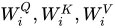 , and
, and are parameter matrices.
The permutation properties of the (standard, unmasked) QKV attention mechanism apply here as well. For permutation matrices, :
: From which we also see that multi-head self-attention:
 is equivariant with respect to permuting the rows of the input matrix.
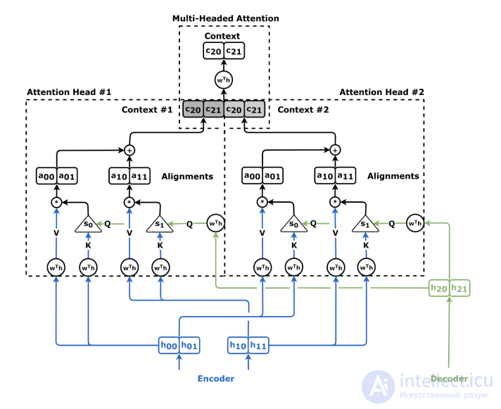
Multi-head cross-attention decoder
 where
where and
and are trainable weight matrices.
 where
where is a trainable weight matrix.
The self-attention mechanism is essentially similar to the cross-attention mechanism, except that the query, key, and value vectors are drawn from the same model. Both the encoder and the decoder can use self-attention, though with some minor differences.
For encoder self-attention, one can start with a simple encoder without self-attention, such as an “embedding layer”, which simply converts each input word into a vector using a fixed lookup table. This gives a sequence of hidden vectors. These can then be fed into a dot-product attention mechanism to obtain
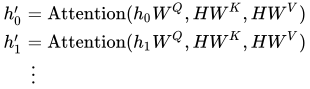 or, more concisely,
 This method can be applied repeatedly to produce a multilayer encoder. This is the so-called “encoder self-attention”, sometimes called “all-to-all attention”, since the vector at every position can attend to every other vector.
For decoder self-attention, “all-to-all” attention is not suitable, since during autoregressive decoding the decoder cannot attend to future outputs that have not yet been decoded. This problem can be solved by forcibly modifying the attention weights. for all
 This attention mechanism is called “causal masking”. It is called “causally masked self-attention”.
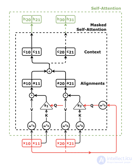
Decoder with self-attention and causal masking, detailed diagram

Comments