Kalman Filter

The Kalman filter is an efficient recursive filter that estimates the state vector of a dynamic system using a series of incomplete and noisy measurements. It is named after Rudolf Kalman.

The Kalman filter is widely used in engineering and econometric applications: from radars and computer vision systems to estimating the parameters of macroeconomic models . Kalman filtering is an important part of control theory and plays a major role in the design of control systems. Together with the linear-quadratic regulator, the Kalman filter makes it possible to solve the linear-quadratic-Gaussian control problem. The Kalman filter and the linear-quadratic regulator are a possible solution to most of the fundamental problems in control theory.

In most applications, the dimension of the object's state vector exceeds the dimension of the observation data vector. Even so, the Kalman filter makes it possible to estimate the complete internal state of the object.

The Kalman filter is designed for recursively refining the estimate of the state vector of an a priori known dynamic system; that is, to calculate the current state of the system one needs to know the current measurement and the previous state of the filter itself. Thus, like other recursive filters, the Kalman filter is implemented in the time domain rather than the frequency domain, but unlike other such filters, it operates not only on state estimates but also on estimates of the uncertainty (the probability density) of the state vector, relying on Bayes' formula for conditional probability.

The algorithm works in two stages. In the prediction stage, the Kalman filter extrapolates the values of the state variables as well as their uncertainties. In the second stage, the extrapolation result is refined using the measurement data (obtained with some error). Thanks to the step-by-step nature of the algorithm, it can track the state of an object in real time (without looking ahead, using only the current measurements and information about the previous state and its uncertainty).

There is a common misconception that the Kalman filter supposedly requires the input data to have a Gaussian distribution in order to work correctly. In Kalman's original work, the results on the minimum covariance of the filter were obtained on the basis of orthogonal projections, without assuming that the measurement errors are Gaussian . It was then simply shown that, for the special case of Gaussian error distributions, the filter gives an exact estimate of the conditional probability distribution of the system state.

A clear example of the filter's capabilities is obtaining optimal, continuously updated estimates of the position and velocity of some object from a time series of inaccurate measurements of its location. For example, in radar the task is to track a target and determine its position, velocity and acceleration, while the measurement results arrive gradually and are very noisy. The Kalman filter uses a probabilistic model of the target's dynamics, which specifies the type of likely motion of the object; this reduces the effect of noise and yields good estimates of the object's position at a present, future or past moment in time.

Introduction

The Kalman filter operates with the concept of the state vector of a system (a set of parameters describing the state of the system at some moment in time) and its statistical description. In the general case, the dynamics of a state vector are described by the probability densities of the distribution of its components at each moment in time. Given a specific mathematical model of the observations made of the system, as well as a model of the a priori change of the state vector parameters (namely, as a Markov shaping process), one can write an equation for the a posteriori probability density of the state vector at any moment in time. This differential equation is called the Stratonovich equation. The Stratonovich equation cannot be solved in the general case. An analytical solution can be obtained only under a number of restrictions (assumptions):

• Gaussian a priori and a posteriori probability densities of the state vector at any moment in time (including the initial one)
• Gaussian shaping noise
• Gaussian observation noise
• white observation noise
• linearity of the observation model
• linearity of the shaping process model (which, recall, must be a Markov process)

The classical Kalman filter is a set of equations for calculating the first and second moments of the a posteriori probability density (in the sense of the vector of expected values and the matrix of variances, including cross-variances) under these restrictions. Since, for a normal probability density, the expected value and the dispersion matrix completely specify the probability density, one can say that the Kalman filter calculates the a posteriori probability density of the state vector at each moment in time, and therefore fully describes the state vector as a random vector quantity.

The calculated expected values are optimal estimates in the mean-square-error sense, which accounts for its wide use.

There are several varieties of the Kalman filter, which differ in the approximations and tricks that have to be applied to reduce the filter to the form described and to lower its dimension:

• the extended Kalman filter (EKF). It reduces nonlinear observation and shaping-process models by linearization using a Taylor series expansion;
• the unscented Kalman filter (UKF). It is used in problems where simple linearization destroys useful relationships between the components of the state vector. In this case the "linearization" is based on the unscented transform ;
• the Ensemble Kalman filter (EnKF). It is used to reduce the dimension of the problem;
• variants are possible with an additional nonlinear filter that converts non-Gaussian observations to normal ones;
• variants are possible with a "whitening" filter that makes it possible to work with "colored" noise;
• and so on.

In addition, there are analogues of the Kalman filter that use a continuous-time model fully or partially:

• the Kalman–Bucy filter, in which both the evolution of the system and the measurements take the form of functions of continuous time;
• the hybrid Kalman filter, which uses continuous time to describe the evolution of the system and discrete moments in time for the measurements.

Historical overview and names

The filter is named after the Hungarian-born mathematician Rudolf E. Kalman, who emigrated to the United States, although Thorvald Nicolai Thiele and Peter Swerling developed a similar algorithm earlier (Thiele considered only a particular special formulation, while Swerling's algorithm is practically identical to Kalman's). Richard S. Bucy of the University of Southern California contributed to the theory that led to the so-called Kalman–Bucy filter. Stanley F. Schmidt^[en] is considered to be the first to implement the Kalman filter, during Kalman's visit to the Ames Research Center, where Kalman saw that his ideas were applicable to the problem of trajectory estimation for the Apollo program, which ultimately led to the inclusion of this filter in the Apollo navigation computer. The Kalman filter was first described and partially developed in the works of Swerling (1958), Kalman (1960) and Kalman and Bucy (1961).

Kalman filters proved to be critically important for the implementation of the navigation systems of US Navy nuclear ballistic missile submarines and in the navigation systems of cruise missiles such as the Tomahawk. It was also used in the navigation and control systems of NASA's Space Shuttle project, and is used in the control and navigation systems of the ISS.

The digital Kalman filter is sometimes called the Stratonovich–Kalman–Bucy filter, because it is a special case of a more general nonlinear filter developed somewhat earlier by the Soviet mathematician R. L. Stratonovich . In fact, some of the equations for special cases of the linear filter appeared in these works of Stratonovich, published before the summer of 1960, when Kalman met Stratonovich during a conference in Moscow.

The dynamic system model used

Kalman filters are based on linear dynamic systems discretized in time. Such systems are modeled as Markov chains using linear operators and terms with a normal distribution. The state of the system is described by a finite-dimensional vector, the state vector. At each time step, a linear operator acts on the state vector and transforms it into another state vector (a deterministic change of state); a normally distributed noise vector (random factors) is added and, in the general case, a control vector that models the influence of the control system. The Kalman filter can be regarded as an analogue of hidden Markov models, with the difference that the variables describing the state of the system are elements of an infinite set of real numbers (as opposed to the finite state-space set in hidden Markov models). In addition, hidden Markov models can use arbitrary distributions for subsequent values of the state vector, unlike the Kalman filter, which uses a normally distributed noise model. There is a strict relationship between the equations of the Kalman filter and those of the hidden Markov model. A review of these and other models is given by Roweis and Ghahramani (1999).

To use the Kalman filter to obtain estimates of a process's state vector from a series of noisy measurements, one must represent the model of that process in accordance with the structure of the filter, as a matrix equation of a certain type. For each step k of the filter's operation, the following matrices must be defined as described below: the process evolution matrix F_k; the observation matrix H_k; the process covariance matrix Q_k; the measurement noise covariance matrix R_k; and, if control inputs are present, the matrix of their coefficients B_k.

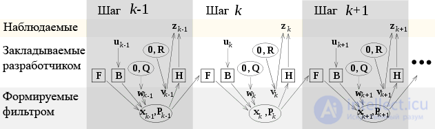
Illustration of the filter's operation. Squares mark matrices. Ellipses mark matrices of multivariate normal distributions (including means and covariances). Vectors are left unenclosed. In the simplest case, some matrices do not change over time (do not depend on the index k), but they are still used by the filter at each step of its operation.

The model of the system (process) implies that the true state at time k is obtained from the true state at time k−1 according to the equation

,

where

• F_k is the system (process) evolution matrix, which acts on the vector x_k−1 (the state vector at time k−1);
• B_k is the control matrix, which is applied to the vector of control inputs u_k;
• w_k is a normal random process with zero expected value and covariance matrix Q_k, which describes the random nature of the evolution of the system (process):

At time k an observation (measurement) z_k of the true state vector x_k is made; the two are related by the equation

,

where H_k is the measurement matrix relating the true state vector to the vector of measurements made, and v_k is white Gaussian measurement noise with zero expected value and covariance matrix R_k:

The initial state and the random process vectors at each step {x₀, w₁, …, w_k, v₁, …, v_k} are assumed to be independent.

Many real dynamic systems cannot be described exactly by this model. In practice, dynamics not accounted for in the model can seriously degrade the performance of the filter, especially when dealing with an unknown stochastic input signal. Moreover, dynamics not accounted for in the model can make the filter unstable. On the other hand, independent white noise as a signal will not cause the algorithm to diverge. The problem of separating measurement noise from dynamics not accounted for in the model is difficult; it is addressed with the help of robust control theory.

The Kalman filter

The Kalman filter is a kind of recursive filter. To compute the estimate of the system state at the current step, it needs the state estimate (in the form of an estimate of the system state and an estimate of the error in determining that state) from the previous step and the measurements at the current step. This property distinguishes it from batch filters, which require knowledge of the history of measurements and/or estimates at the current step. Below, the notation will denote the estimate of the true vector x at time n given the measurements from the start of operation up to and including time m.

The state of the filter is specified by two variables:

• is the a posteriori estimate of the object's state at time k, obtained from observations up to and including time k (in Russian-language literature it is often denoted , where ^ means "estimate" and k is the number of the step at which it was obtained);
• is the a posteriori error covariance matrix, which specifies the accuracy of the obtained state vector estimate and includes estimates of the variances of the error in the computed state and covariances showing the identified relationships between the parameters of the system state (in Russian-language literature it is often denoted ).

Each iteration of the Kalman filter is divided into two phases: extrapolation (prediction) and correction. During extrapolation, the filter obtains a preliminary estimate of the system state (in Russian-language literature it is often denoted , where ~ means "extrapolation" and k is the number of the step at which it was obtained) for the current step from the final state estimate of the previous step (or a preliminary estimate for the next step from the final estimate of the current step, depending on the interpretation). This preliminary estimate is also called the a priori state estimate, since the observations of the corresponding step are not used to obtain it. In the correction phase, the a priori extrapolation is supplemented with the corresponding current measurements to correct the estimate. The corrected estimate is also called the a posteriori state estimate, or simply the estimate of the state vector . Usually these two phases alternate: extrapolation is performed from the results of correction until the next observation, and correction is performed together with the observations available at the next step, and so on. However, another course of events is possible: if for some reason an observation turns out to be unavailable, the correction step can be skipped and extrapolation performed from the uncorrected estimate (the a priori extrapolation). Similarly, if independent measurements are available only at certain steps, corrections are still possible (usually using a different observation matrix H_k).

Next, we consider the operation of the classical optimal Kalman filter.

Extrapolation stage

Extrapolation (prediction) of the system state vector from the state estimate and the applied control vector, from step (k−1) to step k:
Covariance matrix of the extrapolated state vector:

Correction stage

Deviation of the observation obtained at step k from the observation expected given the extrapolation made:
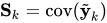
Covariance matrix of the deviation vector (the error vector):
The Kalman-optimal gain matrix, formed from the covariance matrices of the existing state-vector extrapolation and of the measurements obtained (by means of the covariance matrix of the deviation vector):
Correction of the previously obtained state-vector extrapolation — obtaining the estimate of the system state vector:
Calculation of the covariance matrix of the system state-vector estimate:

The expression for the covariance matrix of the system state-vector estimate is valid only when the optimal gain vector given above is used. In the general case this expression has a more complicated form.

Invariants

If the model is absolutely accurate and the initial conditions and are specified absolutely accurately, then the following quantities are preserved after any number of iterations of the filter, that is, they are invariants:

The expected values of the estimates and extrapolations of the system state vector and of the error matrices are zero vectors:

where is the expected value of .

The calculated covariance matrices of the extrapolations, of the system state estimates and of the error vector coincide with the true covariance matrices:

Example of building a filter

Imagine a cart standing on infinitely long rails with no friction. Initially it is at rest at position 0, but under the action of random factors it acquires a random acceleration. We measure the position of the cart every ∆t seconds, but the measurements are inexact. We want to obtain estimates of the cart's position and its velocity. Applying the Kalman filter to this problem, we define all the necessary matrices.

In this problem the matrices F, H, R and Q do not depend on time, so we omit their indices.

The position and velocity of the cart are described by a vector in a linear state space

where is the velocity (the first derivative of the coordinate with respect to time).

We assume that between the (k−1)-th and k-th steps the cart moves with a constant acceleration a_k, normally distributed with zero expected value and standard deviation σ_a. In accordance with Newtonian mechanics we can write

where

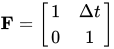
The control matrix is written in the form of a vector

.

The control vector degenerates into the scalar a_k.

The covariance matrix of the random influences

(σ_a is a scalar).

At each step of operation the position of the cart is measured. Suppose that the measurement error v_k has a normal distribution with zero expected value and standard deviation σ_z. Then

,

where

,

and the covariance matrix of the observation noise has the form

.

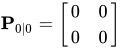
The initial position of the cart is known exactly:

,

.

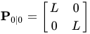
If the position and velocity of the cart are known only approximately, then the variance matrix can be initialized with a sufficiently large number L, so that this number exceeds the variance of the coordinate measurements:

,

.

In this case, during the first steps of operation the filter will give more weight to the measurement results than to the available prior information.

Derivation of the formulas

Covariance matrix of the state-vector estimate

By the definition of the covariance matrix, P_k|k

.

We substitute the expression for the state-vector estimate

and expand the expression for the error vector

and for the measurement vector

.

We factor out the measurement error vector v_k

.

Since the measurement error vector v_k is uncorrelated with the other arguments, we obtain the expression

.

In accordance with the properties of the covariance of vectors, this expression is transformed to the form

.

Replacing the expression for the covariance matrix of the state-vector extrapolation with P_k|k−1 and the definition of the covariance matrix of the observation noise with R_k, we obtain

.

The resulting expression is valid for an arbitrary gain matrix, but if the Kalman-optimal gain matrix is used, this expression for the covariance matrix can be simplified.

Optimal gain matrix

The Kalman filter minimizes the sum of the squared expected values of the state-vector estimation errors.

The error vector of the state-vector estimate

.

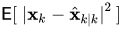
The task is to minimize the sum of the expected values of the squares of the components of this vector:

,

which is equivalent to minimizing the trace of the covariance matrix of the state-vector estimate P_k|k. We substitute the available expressions into the expression for the covariance matrix of the state-vector estimate and complete the square:

		.

Note that the last term is the covariance matrix of some random variable, so its trace is non-negative. The minimum of the trace is reached when the last term vanishes:

This matrix is claimed to be the sought one: when used as the gain matrix in the Kalman filter, it minimizes the sum of the mean squared errors of the state-vector estimate.

Covariance matrix of the state-vector estimate when the optimal gain matrix is used

The expression for the covariance matrix of the state-vector estimate P_k|k when the optimal gain matrix is used takes the form:

This formula is computationally simpler and is therefore used almost always in practice, but it is correct only when the optimal gain matrix is used. If, because of low numerical precision, a problem with numerical stability arises, or if a gain matrix other than the optimal one is deliberately used, the general formula for the covariance matrix of the state-vector estimate should be used.

Kalman–Bucy filter

The Kalman–Bucy filter (named after Richard Snowden Bucy) is the continuous-time version of the Kalman filter , which relies on the following continuous dynamic state model:

,

.

Here and represent the intensities of the two terms (with white-noise characteristics) and , respectively.

The filter consists of two differential equations, one of which serves to estimate the system state and the other to estimate the covariance:

,

where the Kalman gain is obtained by the formula

.

Note that in the expression for the observation-noise covariance represents at the same time the covariance of the prediction error , and these covariances are equal only in the continuous-time case .

The distinction between the prediction and correction steps in discrete Kalman filtering does not exist in the continuous case.

The second differential equation, for the covariance, is an example of a Riccati equation.

Hybrid Kalman filter

Most physical systems have a continuous-time model for the evolution of the system state and a discrete-time measurement model for refining the state. Therefore the filter model can be represented as follows:

,

where

.

Initialization

Prediction

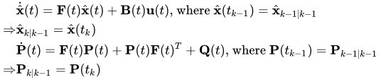
The prediction equations are taken from the continuous-time Kalman–Bucy filter with the measurement term equal to zero . The predicted state and covariance are obtained by integrating the differential equations with the initial value taken from the previous correction step.

Correction

The correction equations are identical to those of the discrete Kalman filter.

Criticism of the Kalman filter

At present, the main criticism of the Kalman filter proceeds along the following lines^[14]:

• In the Kalman filter, errors are represented by white noise, which in fact does not exist in nature.
• It does not satisfy the necessary and sufficient condition of optimality

for t

• There is an error in the derivation of the Kalman filter — contradictory conditions are required for the validity of different equations of the algorithm: in some, that τ < t, and in others τ = t.

Accordingly, the position of the proponents of this filter's optimality is that :

• It is possible to construct a modified Kalman filter in which the errors are represented by colored noise.
• Using the optimality condition in certain cases leads to a less accurate result than the one used in the Kalman filter.
• In deriving the Kalman filter one can adopt the conditions τ < t, τ → t, which removes the contradiction.

Where it is used

• Attitude and heading reference systems
• Autopilot
• Navigation systems:
  • Inertial
  • Terrain-referenced (using digital terrain maps)
  • Satellite

See also

• Marelei's theorem
• Mathematical model of a linear system with a Markov structure
• State prediction of a linear system with a Markov structure
• Correction of state estimates of a linear system with a Markov structure