
Lecture 39 min.
When Schrödinger first discovered the correct laws of quantum mechanics, he wrote an equation that described the probability amplitude for finding a particle at various places. This equation was very similar to the equations that classical physicists already knew and used to describe the motion of air in a sound wave, the propagation of light, and so on. So in the early development of quantum mechanics, people spent most of their time solving this equation. But at the same time, an understanding began to develop (in particular thanks to Born and Dirac) of the fundamentally new ideas that lay at the foundation of quantum mechanics. As the subject developed further, it became clear that it contains many things that are not directly contained in the Schrödinger equation, such as the spin of the electron and various relativistic phenomena. All courses on quantum mechanics traditionally begin in the same way, repeating the path traveled in the historical development of the subject. First they study classical mechanics for a long time, in order later to understand how the Schrödinger equation is solved. Then they spend just as long obtaining various solutions. And only after a detailed study of this equation do they move on to the "higher" questions, such as the spin of the electron.
At first we, too, thought that the best way to end these lectures would be to show how the equations of classical physics are solved in various complicated cases, such as the description of sound waves in an enclosed space, the types of electromagnetic radiation in cylindrical cavities, and so on. That was the original plan for this course. But then we decided to abandon that plan and instead to give an introduction to quantum mechanics. We came to the conclusion that what are usually called the "higher" parts of quantum mechanics are in fact quite simple. The mathematics needed for this is extremely simple: only simple algebraic operations are required, and no differential equations are needed (or at most the very simplest ones). The only problem is to leap over one obstacle: to accept that we no longer have the right to describe in detail the behavior of particles in space. And that is just what we are going to do: tell you about what are usually called the "higher" parts of quantum mechanics. But I assure you that these are the very simplest (in the full sense of the word), and at the same time the most fundamental, parts of it. Frankly, this is a pedagogical experiment, and, as far as we know, it has never been tried before.
Of course, there is a difficulty here: the quantum-mechanical behavior of things is extremely strange. No one can rely on his everyday experience to give him an intuitive, rough idea of what should happen. So this subject can be presented in two ways: either one can describe rather roughly what happens, reporting more or less in detail what will occur but not formulating exact laws, or one can state the exact laws in their abstract form. But then this abstraction will leave you not knowing what it refers to physically. This way is no good, because it is completely abstract, while the first way leaves an unpleasant aftertaste, because one never knows exactly what is true and what is not. And we do not know how to get around this difficulty. We have already met this problem before [Chaps. 37 and 38 (Vol. 3)]. In Chap. 37 the presentation is relatively rigorous, while in Chap. 38 only a rough description of various phenomena is given. Now we shall try to find a happy medium.
We begin this chapter with some general quantum-mechanical ideas. Some of these statements will be perfectly exact, others exact only in part. In the presentation it will be hard for us to point out which are which, but by the time you finish the book you will yourself understand, looking back, which parts stood up and which turned out to be only a rough explanation. The chapters that follow will not be so imprecise. One of the reasons we try to be as precise as possible in the following chapters is that in this way we can demonstrate one of the most beautiful properties of quantum mechanics: how much of it can be deduced from so little.
We again begin by clarifying the properties of the superposition, the addition, of probability amplitudes. As an example we refer to the experiment described in Chap. 37 (Vol. 3) and shown once more here in Fig. 1.1.
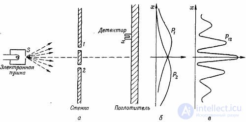
Fig. 1.1. Interference experiment with electrons.
There is a source of particles s, say electrons; beyond it is a wall with two slits in it; behind the wall a detector is placed; it is located somewhere at the point x. We ask: what is the probability that a particle will be detected at the point x? Our first general principle of quantum mechanics is that the probability that a particle leaving the source s will reach the point x can be represented numerically by the square of the modulus of a complex number called the probability amplitude, in our case the "amplitude that a particle from s arrives at x." We shall resort to these amplitudes so often that it will be convenient to use a shorthand notation, invented by Dirac and universally used in quantum mechanics, to represent this concept. We shall write the probability amplitude as follows:

In other words, the two brackets < > are a sign equivalent to the words "the amplitude (of probability) that"; the expression to the right of the vertical bar always gives the starting condition, and what is to the left gives the final condition. Sometimes it will be convenient to abbreviate even further, describing the initial and final conditions by a single letter. For example, amplitude (1.1) can on occasion also be written like this:

It should be emphasized that such an amplitude is, of course, nothing but a number, a complex number.
In Chap. 37 (Vol. 3) we have already seen that when a particle can reach the detector by two paths, the resulting probability is not the sum of two probabilities but must be written as the square of the modulus of the sum of two amplitudes. We found that the probability that the electron reaches the detector with both slits open is

Now we want to write this result in our new notation. First let us state our second general principle of quantum mechanics. When a particle can reach a given state by two possible paths, the total amplitude of the process is the sum of the amplitudes for the two paths considered separately. In our new notation we write

Here we assume that slits 1 and 2 are small enough that when we say the electron passed through a slit, the question of which part of the slit it passed through does not arise. Of course, one could divide each slit into sections, with a finite amplitude that the electron passed through the top of the slit or through the bottom, and so on. We shall assume that the slit is small enough that we do not need to think about this detail. This is one of those imprecisions we spoke of; the matter can be made more precise, but for the time being we shall not do so.
Now we want to spell out in more detail what can be said about the amplitude of the process in which the electron reaches the detector at the point x through slit 1. This can be done by applying a third general principle. When a particle goes along some definite given path, the amplitude for that path can be written as the product of the amplitude that the first part of the path will be traversed and the amplitude that the remainder of the path will be traversed as well. For the setup shown in Fig. 1.1, the amplitude of going from s to x through slit 1 is equal to the amplitude of going from s to 1, multiplied by the amplitude of going from 1 to x:

Again, this statement is not quite accurate. We must add one more factor — the amplitude that the electron passes through the slit at point 1; but for now it is just a slit for us, and we shall set that factor equal to one.
Note that Eq. (1.5) seems to be written backwards. It must be read from right to left: the electron goes from s to 1 and then from 1 to x. In sum, if events occur one after another, that is, if you are able to analyze one of the particle's paths by saying that it first does this, then that, then something else, the resulting amplitude for that path is calculated by successively multiplying by the amplitude of each subsequent event. Using this law, we can rewrite Eq. (1.4) as:

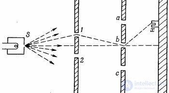
Fig. 1.2. A more complicated interference experiment.
Now we shall show that, using only these principles, we can already solve more difficult problems, such as the one shown in Fig. 1.2. Here two walls are drawn: one with two slits, 1 and 2, the other with three — a, b and c. Behind the second wall, at point x, stands a detector, and we want to know the amplitude that the particle reaches x. One way to solve this is to calculate the superposition, or interference, of the waves passing through the slits; but we can do it differently, by saying that there are six possible paths and superposing their amplitudes. The electron could go through slit 1, then through slit a and then to x, or it could go through slit 1, then through slit b and then to x, and so on. According to our second principle, the amplitudes of mutually exclusive paths add, so we must write the amplitude of the transition from s to x as a sum of six separate amplitudes. On the other hand, according to the third principle, each of them can be written as a product of three amplitudes. For example, one of them is the amplitude of the transition from s to 1, multiplied by the amplitude of the transition from 1 to a and by the amplitude of the transition from a to x. Using our shorthand notation, the total amplitude of the transition from s to x can be written as

We can save space by using the summation sign:

To carry out any calculations with this method, we naturally need to know the amplitude of a transition from one place to another. I shall give an example of a typical amplitude. It leaves out some details, such as the polarization of light or the spin of the electron, but otherwise it is absolutely exact. With it you will be able to solve problems involving various combinations of slits. Suppose that a particle with a definite energy goes through empty space from position r1 to position r2. In other words, it is a free particle: no forces act on it. Dropping the numerical factor in front, the amplitude of the transition from r1 to r2 can be written as

where r12 = r2 — r1, and p is the momentum of the particle, related to its energy E by the relativistic equation
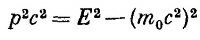
or by the nonrelativistic equation

Equation (1.7) ultimately asserts that the particle has wave properties, that the amplitude propagates like a wave with a wave number equal to the momentum divided by h.
In the general case, time also enters the amplitude and the corresponding probability. In most of our initial discussions it will be assumed that the source emits particles of a given energy continuously, so that there is no need to think about time. But, generally speaking, we may be interested in other questions as well. Suppose that a particle is emitted at some place P at some moment and you want to know the amplitude that it will be at some place, say r, at a later time. This can be represented symbolically as the amplitude <r, t = t1 | P, t = 0>. And it is clear that it depends on both r and t. By placing the detector at different places and making measurements at different moments of time, you will get different results. This function of r and t, generally speaking, satisfies a differential equation which is a wave equation. In the nonrelativistic case, for instance, this is the Schrödinger equation. What results is a wave equation analogous to the equation for electromagnetic waves or for sound waves in a gas. However, it must be emphasized that the wave function satisfying the equation is not like a real wave in space; no reality can be associated with this wave, as is done with a sound wave.
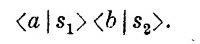
Although, when dealing with a single particle, one can begin to try to think in the language of "particle waves," there is nothing good in it, because if, say, there are not one but two particles, then the amplitude to find one of them at r1 and the other at r2 is not an ordinary wave in three-dimensional space, but depends on six spatial variables, r1 and r2. When there are two (or more) particles, the need arises for the following additional principle. If two particles do not interact, then the amplitude that one particle does one thing and the other does something else is the product of two amplitudes — the amplitudes that the two particles would do it separately. For example, if <a | s1> is the amplitude that particle 1 goes from s1 to a, and <b | s2> is the amplitude that particle 2 goes from s2 to b, then the amplitude that both of these events occur together is
One more thing must be emphasized. Suppose we do not know where the particles in Fig. 1.2 come from before they pass through slits 1 and 2 in the first wall. Nevertheless, we can still predict what will happen behind the wall (say, calculate the amplitude to arrive at x), provided we are given two numbers: the amplitude to arrive at 1 and the amplitude to arrive at 2. In other words, because the amplitudes of successive events are multiplied, as shown in Eq. (1.6), all you need to know to continue the analysis is these two numbers, in this particular case <1 | s> and <2 | s>. These two complex numbers are enough to predict the whole future. This is what makes quantum mechanics simple. In the following chapters it will become clear that this is exactly what we do when we specify the initial conditions by means of two (or several) numbers. Of course, these numbers depend on where the source is located and on the other properties of the apparatus, but once these numbers are given, we no longer need any such details.
Let us consider once more a question that we discussed in considerable detail earlier, in Chap. 37 (Vol. 3). Now we shall use the idea of the amplitude in all its power, to show you how it works. Let us return to the old experiment shown in Fig. 1.1, adding to it a light source placed behind the slits (cf. Fig. 37.4 of Chap. 37). In Chap. 37 we found the following remarkable result. If we looked behind slit 1 and noticed photons scattered somewhere behind it, then the probability distribution of the electron arriving at x, while these photons were simultaneously observed, was exactly the same as if slit 2 were closed. The total distribution for electrons that were "noticed" either at slit 1 or at slit 2 was the sum of the separate distributions and was quite unlike the distribution obtained when the light was turned off. At least this was so when light of short wavelength was used. When the wavelength began to increase and we lost certainty about at which slit the light scattering had occurred, the distribution became similar to the one obtained with the light turned off.
Let us now see what happens here, using our new notation and the principles of composition of amplitudes. To simplify the writing, we can again denote by φ1 the amplitude that the electron arrives at x through slit 1, that is,
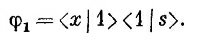
Similarly, φ2 will denote the amplitude that the electron reaches the detector through slit 2:
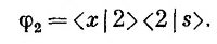
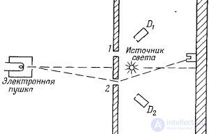
These are the amplitudes for the electron to penetrate through a slit and appear at x when there is no light. But if the light is on, we pose ourselves the question: what is the amplitude of the process in which at the start the electron leaves s and a photon is emitted by the light source L, and at the end the electron is at x and the photon is detected at slit 1? Suppose that with the help of counter D1 we observe a photon at slit 1 (Fig. 1.3), while an identical counter D2 counts photons scattered at slit 2. Then we can speak of the amplitude of a photon appearing in counter D1 and an electron at x, and of the amplitude of a photon appearing in counter D2 and an electron at x. Let us try to calculate them.
Although we do not have the correct mathematical formula for all the factors entering this calculation, you will get the spirit of the calculation from the following reasoning. First, there is the amplitude <1 | s> that the electron gets from the source to slit 1. Then we can suppose that there is a finite amplitude that, when the electron is at slit 1, it scatters a photon into counter D1. Let us denote this amplitude by a. Then there is the amplitude <x | 1> that the electron goes from slit 1 to the electron counter at x. The amplitude that the electron goes from s to x through slit 1 and scatters a photon into counter D1 is then equal to
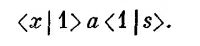
Or, in our earlier notation, it is simply aφ1.
There is also some amplitude that an electron passing through slit 2 scatters a photon into counter D1. You will say: "This is impossible; how can it scatter into counter D1 if that counter looks straight at slit 1?" If the wavelength is large enough, diffraction effects appear, and this becomes possible. Of course, if the apparatus is built well and if only photons of short wavelength are used, the amplitude that a photon is scattered into counter D1 by an electron at slit 2 will be very small. But for the generality of the argument we shall take into account the fact that such an amplitude always exists, and denote it by b. Then the amplitude that the electron passes through slit 2 and scatters a photon into counter D1 is

The amplitude of finding the electron at x and the photon in counter D1 is the sum of two terms, one for each conceivable path of the electron. Each of them in turn is composed of two factors: the first, expressing that the electron passed through the slit, and the second, that the photon was scattered by such an electron into counter D1; we have

A similar expression can be obtained for the case when the photon is detected by the other counter, D2 . If we assume for simplicity that the system is symmetric, then a will also be the amplitude for the photon to reach counter D2 when the electron slips through slit 2, and b the amplitude for the photon to reach counter D2 when the electron passes through slit 1. The corresponding total amplitude — the amplitude that the photon will be in counter D2 and the electron at x — is equal to

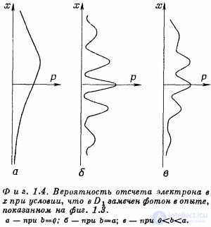
That is all. Now we can easily calculate the probability of one case or another. Say we want to know with what probability counts will be obtained in counter D1 when the electron arrives at x. This will be the square of the modulus of the amplitude given by formula (1.8), that is, simply | aφ1 + bφ2 |2. Let us look at this expression more closely. First of all, if b = 0 (we would like our apparatus to work exactly this way), the answer is simply equal to | φ1|2 with the factor | a |2. This is just the probability distribution that would be obtained with only one slit, as shown in Fig. 1.4, a. On the other hand, if the wavelength is large, the scattering behind slit 2 into counter D1 can become almost the same as behind slit 1. Although some phases may enter a and b, let us take the simplest case, when both phases are the same. If a practically coincides with b, then the total probability becomes | φ1 + φ1 |2 multiplied by | a |2, because the common factor a can be taken out. But then we get the very probability distribution that would be obtained if there were no photons at all. Consequently, when the wavelength is very large (and detecting photons is useless), you return to the original distribution curve, in which interference effects are visible, as shown in Fig. 1.4, b. When the detection is nevertheless partially effective, interference arises between a large amount of φ1 and a small amount of φ2, and you get an intermediate distribution, such as the one sketched in Fig. 1.4, c. It goes without saying that if we are interested in simultaneous counts of photons in counter D2 and electrons at x, we shall get the same result. If you recall the discussion of Chap. 37 (Vol. 3), you will see that these results describe quantitatively what was said there.
We would like to stress a very important point and to warn against a frequently made mistake. Suppose you are interested only in the amplitude that the electron arrives at x, and you do not care which counter the photon went into — D1 or D2. Should you add the amplitudes (1.8) and (1.9)? No! Never add amplitudes for different, distinct final states. Once the photon has been registered by one of the photon counters, we can always, if necessary, find out, without disturbing the system any further, which of the alternatives (mutually exclusive events) was realized. Each alternative has its own probability, completely independent of the other. We repeat: do not add amplitudes for different final conditions (by "final" we mean the moment when we are interested in the probability, that is, when the experiment is "finished"). But you must add the amplitudes for different indistinguishable alternatives in the course of the experiment itself, before the process is completely finished. At the end of the process you may, if you like, say that you "do not wish to look at the photon." That is your personal affair, but the amplitudes still cannot be added. Nature does not know what you are looking at and what you are not; it behaves as it is supposed to, and it is indifferent to whether you are interested in its data or not. So we must not add amplitudes. We first square the moduli of the amplitudes for all the possible different final states, and only then add. The correct result for an electron at x and a photon in either D1 or D
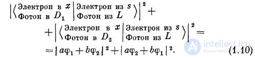
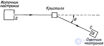
Fig. 1.5. Measurement of neutron scattering from a crystal.
The next example is a phenomenon in which the interference of probability amplitudes must be analyzed more carefully. It concerns the process of neutron scattering from a crystal. Suppose we have a crystal containing many atoms, with a nucleus at the center of each atom; the nuclei are arranged periodically, and a beam of neutrons comes at them from somewhere far away. The various nuclei in the crystal can be numbered by an index ¡, where i runs through the integer values 1, 2, 3, ... , N, and N is the total number of atoms. The task is to calculate the probability that a neutron will be found in the counter shown in Fig. 1.5. For each individual atom i, the amplitude that the neutron reaches counter C is equal to the amplitude that the neutron from source S gets to nucleus ¡, multiplied by the amplitude a of scattering at that place and multiplied by the amplitude that it gets from i to counter C. Let us write this down:

In writing this we assumed that the scattering amplitude a is the same for all atoms. Here we have a multitude of apparently indistinguishable paths. They are indistinguishable because a neutron of low energy scatters from a nucleus without knocking the atom itself out of its place in the crystal — no "mark" of the scattering is left. According to our earlier discussion, the total amplitude that the neutron got into C includes the sum of expression (1.11) over all atoms:

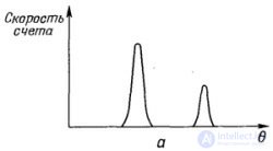
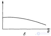
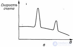
Fig.1.6. Neutron count rate as a function of angle. a — for nuclei with spin 0; b — probability of scattering with spin flip; c — observed count rate for a nucleus with spin 1/2.
Because the scattering amplitudes from atoms located differently in space are added, the amplitudes will have different phases, and this will give a characteristic interference pattern, which we have already analyzed in the example of the scattering of light from a grating.
The intensity of neutrons as a function of angle in such an experiment does often show very strong variations — very sharp interference peaks with nothing between them (Fig. 1.6, a). However, in some kinds of crystals this does not happen; in them, along with the diffraction peaks mentioned above, there is a general background of scattering in all directions. We must try to understand the seemingly mysterious reason for this. The point is that we have not taken into account one important property of the neutron. Its spin is 1/2, and so it can be in two states: either its spin points up (say, across the page in Fig. 1.5), or down. And if the nuclei of the crystal itself have no spin, the spin of the neutron will have no effect. But when the nuclei of the crystal also have a spin, equal, say, also to 1/2, you will notice a background from the smeared scattering described above. The explanation is as follows.
If the spin of the neutron points in some direction and the spin of the atomic nucleus points the same way, then in the scattering process the direction of the spin does not change. If, however, the spins of the neutron and of the atomic nucleus point in opposite directions, then scattering can occur by means of two processes, in one of which the directions do not change, and in the other of which the directions are exchanged. This rule that the sum of the spins must not change is analogous to our classical law of conservation of angular momentum. And we shall be able to understand the phenomenon of interest if we assume that all the nuclei on which scattering occurs have the same spin direction. A neutron with the same spin direction will then scatter so as to give the expected narrow interference distribution. But what happens to a neutron with the opposite spin direction? If it scatters without flipping its spin, nothing changes compared with what has been said; but if both spins flip in the scattering, then, generally speaking, one can indicate at which nucleus the scattering occurred, because it is precisely this nucleus whose spin has flipped. But if we are able to indicate at which atom the scattering happened, then what do the remaining atoms have to do with it? Nothing, of course. The scattering here is the same as from a single atom.
To take this effect into account, we must modify the mathematical formulation of Eq. (1.12), because in that analysis the states were not fully characterized. Let initially all the neutrons leaving the source have their spin pointing up, and all the nuclei of the crystal have theirs pointing down. First, we need the amplitude that in the neutron counter their spin will be pointing up and all the spins in the crystal will still be pointing down. This is no different from our earlier discussion. Let us denote by a the amplitude of scattering without spin flip. The amplitude of scattering from the i-th atom is, of course, equal to

Since all the atomic spins point down, the different alternatives (different values of i) cannot be distinguished from one another. In this process all the amplitudes interfere.
But there is also another case, when the spin of the detected neutron points down, although at the beginning, at S, it pointed up. Then in the crystal one of the spins must flip up, say the spin of the k-th atom. Suppose that for all atoms the amplitude of scattering with spin flip is the same and equal to b. (In a real crystal there is one more unpleasant possibility: the flipped spin passes to some other atom, but let us assume that in our crystal the probability of this is small.) Then the scattering amplitude is

If we now ask what the probability is that the neutron's spin will be pointing down and that of the k-th nucleus up, it will be equal to the square of the modulus of this amplitude, that is, simply |b|2 multiplied by | <C | k> <k | S > |2. The second factor hardly depends on where atom k is located in the crystal, and all the phases disappear when the square of the modulus is calculated. The probability of scattering with spin flip from any nucleus of the crystal is therefore equal to

which gives a smooth distribution, as in Fig. 1.6, b.
You may object: "I don't care which atom flipped." Be that as it may, nature knows it, and the probability actually turns out to be as written above — no interference is left. But if you are interested in the probability that the spin in the detector will point up while the spins of all the atoms still point down, then you must take the square of the modulus of the sum:
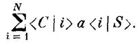
Since each term in this sum has its own phase, they interfere and a sharp interference pattern appears. And if we carry out an experiment in which we do not observe the spin of the detected neutron, then events of both types can occur and the separate probabilities will be added. The total probability (or count rate) as a function of angle then looks like the curve in Fig. 1.6, c.
Let us once more survey the physics of this experiment. If you are able in principle to distinguish mutually exclusive final states (even though you did not actually intend to do so), then the total final probability is obtained by calculating the probability of each state (not the amplitude) and then adding them. But if you are unable, even in principle, to distinguish the final states, then you must first add the probability amplitudes, and only then calculate the square of the modulus and find the probability itself. Note especially that if you tried to picture the neutron as a single wave, you would get the same distribution both for the scattering of neutrons with spin down and for neutrons with spin up. You would have to say that the "wave" of neutrons with spin pointing down came from all the different atoms and interferes in the same way as the wave of neutrons of the same wavelength with spin pointing up. But we know that in fact this is not so. So (as we have already noted) one must be careful not to picture waves in space too realistically. They are useful for some problems. But not for all.
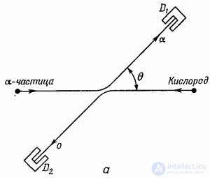
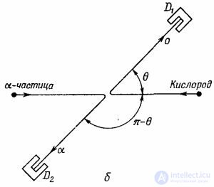
Fig. 1.7. Scattering of α-particles from oxygen nuclei, observed in the center-of-mass system.
The next experiment we want to describe will demonstrate one of the remarkable consequences of quantum mechanics. Here we again meet physical events in which there are two indistinguishable paths and, as always in such circumstances, interference of amplitudes arises. We are going to consider the scattering of some nuclei from other nuclei at relatively low energy. Let us begin, say, with α-particles (which, as you know, are simply helium nuclei) bombarding oxygen. To make the analysis of the reaction easier, we carry it out in the center-of-mass system, in which the velocities of the oxygen nucleus and the α-particle before the collision are opposite, and after the collision are also opposite (Fig. 1.7, a). (The magnitudes of the velocities are, of course, different, since the masses are different.) Let us also assume that energy is conserved and that the collision energy is so small that the particles neither break up nor go into an excited state. The reason the particles deflect each other is simply that both are positively charged and, speaking classically, repel each other as they pass by. Scattering to different angles will occur with different probabilities, and we want to find out the angular dependence of such scattering. (Of course, all this can be calculated classically, and by a remarkable coincidence it turns out that the answer to this question is the same in quantum mechanics and in classical mechanics. This is very curious, because for no force law other than the inverse-square law is this so, so it really is a coincidence.)
The probability of scattering in various directions can be measured in the experiment shown in Fig. 1.7, a. Counter D1 can be designed to detect only α-particles; counter D2 can be set up to detect oxygen, simply as a check. (In the center-of-mass system the detectors must face each other; in the laboratory system they need not.) The experiment consists of measuring the probability of scattering in various directions. Let f (θ) denote the amplitude for scattering into the counters when they are placed at angle θ; then | f (θ) |2 is our experimentally determined probability.
We could also carry out another experiment, in which our counters would respond to both the α-particle and the oxygen nucleus. Then we need to work out what happens if we decide not to care which of the particles entered the counter. Of course, when the oxygen goes off in the direction θ, an α-particle must appear on the opposite side, at angle (π — θ) (Fig. 1.7, b). So if f (θ) is the amplitude for scattering of oxygen through angle θ, then f (π — θ) is the amplitude for scattering of the α-particle through angle θ. Thus the probability that some particle will end up in the counter located at position D1 is

Note that in principle the two states are distinguishable. Even if we did not distinguish them in this experiment, we could have done so. And in accordance with our earlier reasoning, we must therefore add probabilities, not amplitudes.
The result above holds for many nuclei. The target may be oxygen, carbon, beryllium, or hydrogen. But it is wrong for the scattering of α-particles by α-particles. In that one case, when the two particles are exactly identical, the experimental data disagree with the predictions of formula (1.14). For example, the probability of scattering through 90° is exactly twice as large as predicted by the theory just described — with particles that are «helium» nuclei, the trick does not work. If the target is He3 and α-particles (He4) are fired at it, all is well. Only when the target is He4, that is, when its nuclei are identical to the incident α-particles, does the scattering vary with angle in some special way.
Perhaps you have already guessed what is going on? An α-particle can end up in the counter for two reasons: either because the incident α-particle was scattered through angle θ, or because it was scattered through angle (π — θ). How can we make sure who entered the counter — the projectile or the target particle? There is no way. In the scattering of α-particles by α-particles there are two alternatives that cannot be told apart. We have to let the probability amplitudes interfere by adding them, and the probability of finding an α-particle in the counter is the square of this sum:

This is quite different from (1.14). Take, say, the angle π/2 (it is easier to picture). At θ = π/2 we naturally have f (θ)= f(π — θ), so from (1.15) the probability turns out to be

On the other hand, if there were no interference, formula (1.14) would give only 2 | f (π/2) |2. So twice as many particles are scattered through 90° as one could expect. Of course, at other angles the results will differ too. And we arrive at an unusual conclusion: when the particles are identical, something new happens that never occurred when the particles could be distinguished from one another. In the mathematical description you must add the amplitudes of mutually exclusive processes in which the two particles simply exchange roles, and interference occurs.
An even more unexpected phenomenon occurs in the scattering of electrons by electrons or protons by protons. Then none of the earlier results is correct! For these particles we must call to our aid a completely new rule: if an electron arriving at some point exchanges its identity with another electron, the new amplitude interferes with the old one out of phase. It is still interference, but with the opposite sign. In the case of α-particles, when the α-particles reaching the counter are exchanged, the amplitudes interfere with the same sign. In the case of electrons, the exchange amplitudes interfere with different signs. Up to one detail, which will be mentioned shortly, the correct formula for electrons in an experiment like the one shown in Fig. 1.8 is:
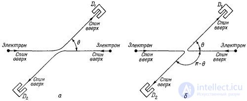
Fig. 1.8. Scattering of electrons by electrons.

This statement needs refinement, because we have not taken into account the spin of the electron (α-particles have no spin). The electron spin can be regarded as pointing either up or down relative to the scattering plane. If the energy in the experiment is low enough, the magnetic forces arising from currents will be small and will not affect the spin. Let us assume in our analysis that this is so, so that there is no chance for the spins to flip in the collision. Whatever spin the electron has, it carries it away with it. We now see that there are many possibilities. For the projectile particle and the target particle, both spins may point up, or down, or in different directions. If both point up, as in Fig. 1.8 (or both point down), then after scattering the same will remain, and the amplitude of the process will be the difference of the amplitudes of the two possibilities shown in Fig. 1.8. The probability of finding an electron in counter D1 will then be given by formula (1.16).
Suppose, however, that the spin of the «projectile» points up and that of the «target» points down. The electron that ends up in counter D1 may have its spin pointing either up or down, and by measuring this spin we can tell whether the electron came out of the bombarding beam or out of the target.
These two possibilities are shown in Fig. 1.9; in principle they are distinguishable, and therefore no interference will result — the two probabilities simply add. All this is also true when both initial spins are reversed, that is, if the spin on the left points down and the spin on the right points up.
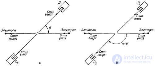
Fig. 1.9. Scattering of electrons with antiparallel spins.
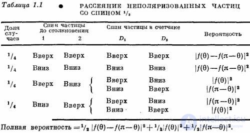
Finally, if the electrons are emitted at random (for example, if they come out of a hot tungsten filament as a completely unpolarized beam), then each individual electron is equally likely to come out with spin up or spin down. If in our experiment we do not intend to measure the spin of the electrons at any point, what we have is what is called an experiment with unpolarized particles. The result of this experiment is best calculated by listing all the conceivable possibilities, as is done in Table 1.1. For each distinguishable alternative the probability is calculated separately. The total probability is then the sum of all the individual probabilities. Note that for unpolarized beams the result at θ = π/2 is half the classical result for independent particles.
The behavior of identical particles leads to many interesting consequences; in the next chapter we will discuss them in more detail.

Comments